Z Score Calculator
Convert a raw value into a standard z score with z = (x – μ) / σ, then read the percentile and normal-curve probability. Reverse a z back to a raw value, or standardize a sample mean using the standard error.
🎯Real Z Score Presets
📝Standardization Inputs
The observed score, measurement, or sample average.
Must be greater than 0. Use the population σ.
Used only when mode is z → raw value.
Standard error = σ / √n for the sample-mean mode.
Group 2 SD. Group 2 sample size below.
🔢Formula Snapshot
📊Z Score to Percentile Table
| z score | P(Z < z) | Percentile | Right tail P(Z > z) | Band vs mean |
|---|---|---|---|---|
| -3.0 | 0.0013 | 0.13th | 0.9987 | Far below |
| -2.5 | 0.0062 | 0.62nd | 0.9938 | Well below |
| -2.0 | 0.0228 | 2.28th | 0.9772 | Below |
| -1.5 | 0.0668 | 6.68th | 0.9332 | Below |
| -1.0 | 0.1587 | 15.87th | 0.8413 | Slightly below |
| -0.5 | 0.3085 | 30.85th | 0.6915 | Near mean |
| 0.0 | 0.5000 | 50.00th | 0.5000 | At the mean |
| 0.5 | 0.6915 | 69.15th | 0.3085 | Near mean |
| 1.0 | 0.8413 | 84.13th | 0.1587 | Slightly above |
| 1.5 | 0.9332 | 93.32nd | 0.0668 | Above |
| 2.0 | 0.9772 | 97.72nd | 0.0228 | Above |
| 2.5 | 0.9938 | 99.38th | 0.0062 | Well above |
| 3.0 | 0.9987 | 99.87th | 0.0013 | Far above |
🎯Common Critical Z Values
| Confidence | Alpha | Two-tailed z | One-tailed z | Typical use |
|---|---|---|---|---|
| 80% | 0.20 | 1.282 | 0.842 | Rough intervals |
| 90% | 0.10 | 1.645 | 1.282 | Screening tests |
| 95% | 0.05 | 1.960 | 1.645 | Standard reporting |
| 98% | 0.02 | 2.326 | 2.054 | Tighter bounds |
| 99% | 0.01 | 2.576 | 2.326 | Clinical / finance |
| 99.9% | 0.001 | 3.291 | 3.090 | Very strict |
📏Empirical Rule (68-95-99.7)
| Range | z bounds | Area inside | Area in tails | Interpretation |
|---|---|---|---|---|
| μ ± 1σ | -1 to +1 | 68.27% | 31.73% | About two-thirds of data |
| μ ± 2σ | -2 to +2 | 95.45% | 4.55% | Vast majority of data |
| μ ± 3σ | -3 to +3 | 99.73% | 0.27% | Nearly all data |
| μ ± 1σ band | -1 to +1 | 68.27% | 31.73% | Live band for your inputs |
| μ ± 2σ band | -2 to +2 | 95.45% | 4.55% | Live band for your inputs |
| μ ± 3σ band | -3 to +3 | 99.73% | 0.27% | Live band for your inputs |
🗂Z Score Interpretation Bands
| z range | Position | Percentile range | Rarity | Example | Flag |
|---|---|---|---|---|---|
| z < -3 | Far below mean | Below 0.1th | About 1 in 740 | Extreme low outlier | Outlier |
| -3 to -2 | Well below mean | 0.1th to 2.3rd | About 1 in 44 | Low score | Unusual |
| -2 to -1 | Below mean | 2.3rd to 15.9th | Roughly 1 in 7 | Lower group | Notable |
| -1 to 0 | Slightly below | 15.9th to 50th | Common | Below average | Typical |
| 0 to 1 | Slightly above | 50th to 84.1th | Common | Above average | Typical |
| 1 to 2 | Above mean | 84.1th to 97.7th | Roughly 1 in 7 | Upper group | Notable |
| 2 to 3 | Well above mean | 97.7th to 99.9th | About 1 in 44 | High score | Unusual |
| z > 3 | Far above mean | Above 99.9th | About 1 in 740 | Extreme high outlier | Outlier |
⚙Full Formula Breakdown
📋Reference: Symbols & Values
| Symbol | Meaning | How it is used | Effect on z |
|---|---|---|---|
| x | Raw value or score | Top of numerator | Higher x raises z |
| μ (mu) | Population mean | Subtracted from x | Higher μ lowers z |
| σ (sigma) | Standard deviation | Divides the gap | Larger σ pulls z toward 0 |
| n | Sample size | Standard error σ/√n | Larger n grows |z| for means |
| z | Standard score | Feeds the normal CDF | Sets percentile and tails |
💡Practical Z Score Tips
Take a standardized test and score an eighty-five. You may be feeling decent about yourself until you see that the class average was seventy, with a tight spread of ten points. Suddenly your eighty-five starts to look pretty good, now you know exactly where it sits on the distribution.
That’s what statisticians refer to as a z-score; this turns raw numbers into relative standing. To do so, you only need to know your mean and standard deviation. Then you can simply plug these values into the calculator above, saving you the hassle of wrestling with probability tables or memorizing complicated formulas. It’s just algebra that tells a story about position and rarity.
What is a Z-Score?
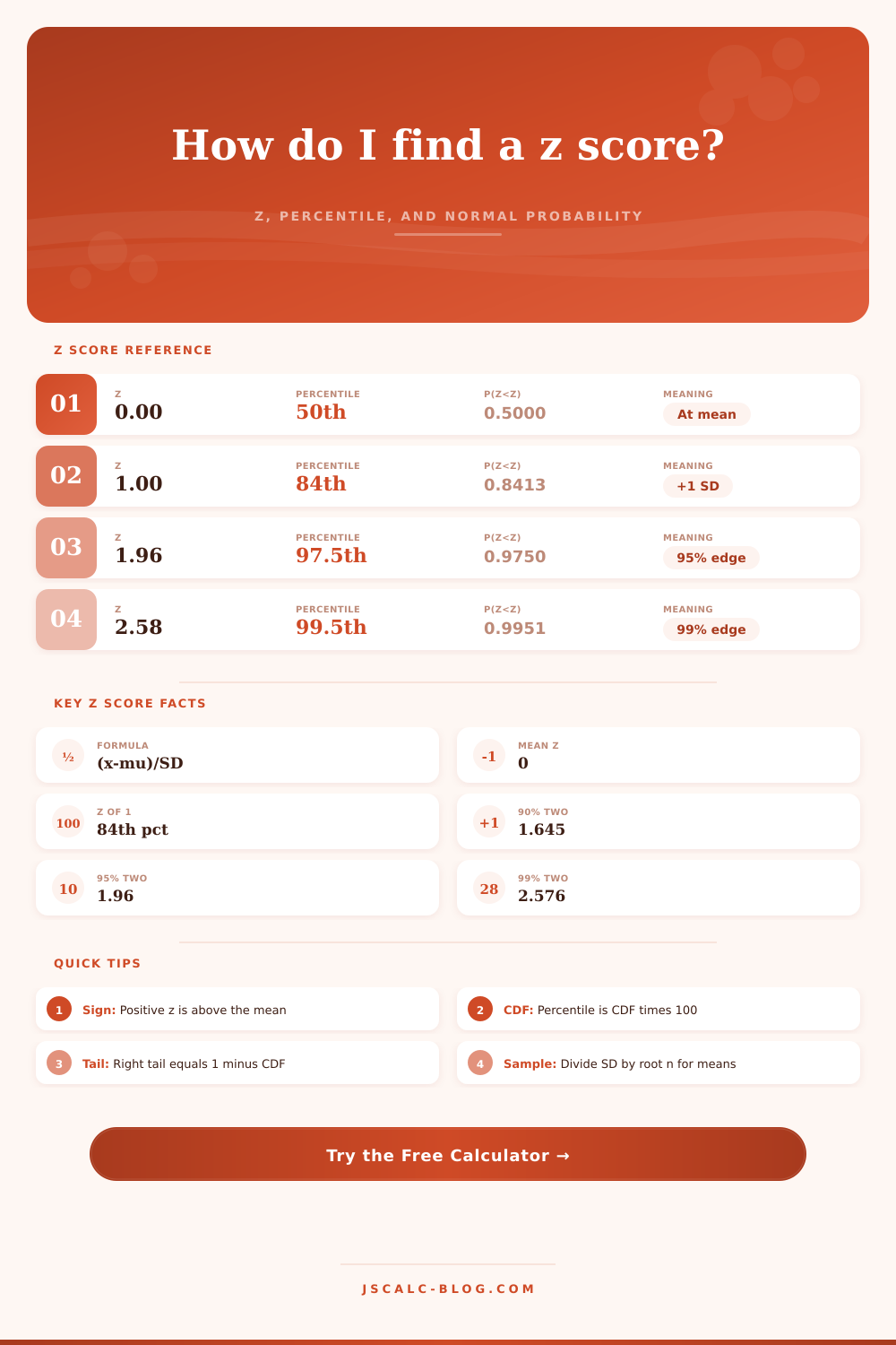
But it turns out that this idea, while incredibly powerful; is also pretty straightforward. A z-score are a way to measure the number of standard deviations by which a given data point differs from the mean of its population. The average is equal to a z-score of zero. If your score was identical to the population norm, you’d be smack dab in the dead-center of the bell curve. This means you’d fall within the range where 50% of the population did better and 50% did worse. You’re literally the epitome of “normal.”
That is boring, unless you remember that most things follow a tight distribution centered around that average. If you have a z-score of +1, then you’re in the eighty-fourth percentile or so. Congratulations! By doing absolutely nothing special, you’re beating most of the competition.
However, few realize that a raw score isn’t the same as statistical significance. Sure, 90 is great if it’s on an easy test, but maybe your test was brutally curved and an 82 has a smaller Z-score. That’s where standard deviation comes into play. Tighter scores means bigger deviations, which means small variations is statistically significant.
That’s what the tool can also help you visualize: both your percentile rank and the CDF (cumulative area under the curve). Seeing a percentile rank like, “you’re in the top 10%” can be far more intuitive than looking at a decimal probability. Seeing that 90% of the area is beneath you can immediately show how out-of-the-ordinary your score actualy is.
Take for example a quality control inspector weighing items from a production line. The average (target) weight is the mean, and the acceptable fluctuation are the standard deviation. Once an item reaches a z-score of two or more, it’s trending towards the fringe of what can be accepted. A three sigma event is an outlier, happening roughly one time out of every 700. And it’s not academic; this is how a factory spots a malfunctioning machine before it costs tens of thousands of dollars worth of junk products.
The empirical rule tells us that nearly everything lies between three standard deviations. Anything beyond that warrants further inspection. The other complication that often throws off both students and pros has to do with sample size. If we’re dealing with an average, not a single observation, then our variability decreases as our sample size increase (this is what’s known as the standard error). That means big studies can pick up small differences that would of been lost on smaller studies.
The calculator takes your sample size into account by altering the formula’s denominator. Oddly, that makes the result less noisy when your sample size are large, even though common sense says that a greater sample size ought to increase noise. Statistically speaking, however, it anchors the estimate down further to the actual mean.
In science, you see numbers like 1.96 pop up all over the place. That’s the cutoff point, or z-score, below which we say something is just random noise and above which we call it a significant effect. Knowing where those numbers originate gives you a healthy dose of skepticism when reading scientific papers. If a paper only just reaches significance, it may not be replicable.
The page provides a reference table that lays it out nicely: the relationship between confidence level and z-score. If you grasp that greater confidence means wider boundaries, you don’t have to remember the numbers themselves.
In the end, what does statistics do? It does not eliminate uncertainty; it manages it. A single data point has a story to tell: What place did it occupy within some bigger pattern? With those standard units, we’re able to make comparisons across categories, like apples and oranges, income level and test score, blood pressure and height. They stop being abstractions with names attached and become points on a map. Where do they sit relative to the mean? That helps us understand a confusing world.
Be it financial risk analysis or exam grading, having this sense of location make sense of it all. It transforms confusion into comparison.