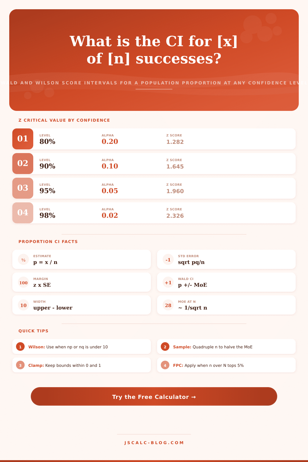
Confidence Interval of Proportion Calculator (Wald & Wilson)

Confidence Interval of a Proportion Calculator

Enter successes x and sample size n, or a decimal sample proportion, then choose a confidence level to compute a confidence interval for the true population proportion. Get both the Wald normal-approximation interval and the more accurate Wilson score interval, plus the standard error, margin of error, z critical value, and interval width, with an optional finite population correction.

🔢Input Mode

🎯Real Study Presets

📝Sample and Confidence Inputs

Successes (x)

Number of items in the sample with the trait of interest.

Sample proportion (p-hat)

Decimal between 0 and 1, for example 0.54 for 54 percent.

Sample size (n)

Total number of observations in the sample.

Confidence level

Sets the two-sided z critical value used for the margin.

Interval method

Drives the primary interval card; both intervals always show below.

Population size N (0 = infinite)

Enter a finite N to apply the finite population correction.

Decimal places

Controls rounding on every result and bound.

Show bounds as

Percent multiplies every proportion output by 100.

Confidence Interval 0 to 0 lower and upper bound

Point Estimate p-hat 0 with margin of error

Standard Error and z 0 SE, z critical value

Interval Width 0 relative margin of error

🧮Formula Snapshot

p̂x / n

SE√(p̂q̂/n)

MoEz × SE

CIp̂ ± MoE

📈z Critical Value by Confidence Level

Confidence Level	Alpha	Alpha / 2	z Critical (two-sided)	Typical Use
80%	0.20	0.10	1.282	Quick internal reads
90%	0.10	0.05	1.645	Exploratory analysis
95%	0.05	0.025	1.960	Standard reporting
98%	0.02	0.01	2.326	Higher assurance
99%	0.01	0.005	2.576	Clinical and finance
99.9%	0.001	0.0005	3.291	Safety-critical claims

📏Approximate Margin of Error at 95% (p-hat = 0.5)

Sample Size n	Std Error	Margin of Error	MoE in Percent	Interval Width
50	0.0707	0.1386	13.9%	0.277
100	0.0500	0.0980	9.8%	0.196
200	0.0354	0.0693	6.9%	0.139
400	0.0250	0.0490	4.9%	0.098
600	0.0204	0.0400	4.0%	0.080
1000	0.0158	0.0310	3.1%	0.062
1500	0.0129	0.0253	2.5%	0.051
2400	0.0102	0.0200	2.0%	0.040

⚖Wald vs Wilson Score Comparison

Data (x / n)	p-hat	Wald 95% CI	Wilson 95% CI	np & nq Check	Better Choice
540 / 1000	0.540	0.509 to 0.571	0.509 to 0.571	540, 460 OK	Either
85 / 100	0.850	0.780 to 0.920	0.767 to 0.911	85, 15 OK	Wilson
12 / 500	0.024	0.011 to 0.037	0.014 to 0.042	12 small	Wilson
2 / 40	0.050	-0.017 to 0.117	0.014 to 0.161	2 tiny	Wilson
495 / 500	0.990	0.981 to 0.999	0.977 to 0.996	5 small	Wilson
320 / 2000	0.160	0.144 to 0.176	0.144 to 0.177	320, 1680 OK	Either
7 / 210	0.033	0.009 to 0.058	0.016 to 0.067	7 small	Wilson
0 / 30	0.000	0.000 to 0.000	0.000 to 0.114	0 fails	Wilson

🗃Interval Width by Confidence and Sample Size (p-hat = 0.5)

Confidence	z	MoE at n=100	MoE at n=400	MoE at n=1000	MoE at n=2000
80%	1.282	0.0641	0.0321	0.0203	0.0143
90%	1.645	0.0822	0.0411	0.0260	0.0184
95%	1.960	0.0980	0.0490	0.0310	0.0219
98%	2.326	0.1163	0.0582	0.0368	0.0260
99%	2.576	0.1288	0.0644	0.0407	0.0288
99.9%	3.291	0.1645	0.0823	0.0521	0.0368

🧭When to Use Each Method

Situation	Recommended	Why	Watch For
Large n, p near 0.5	Wald	Simple and accurate here	None major
np or nq under 10	Wilson	Stays inside 0 and 1	Skewed sampling
p near 0 or 1	Wilson	No impossible bounds	Zero successes
Very small samples	Wilson + cc	Better coverage	Wider interval
Sample over 5% of N	Add FPC	Shrinks the margin	Need known N
Reporting to public	95% level	Widely understood	State the method

⚙Formula Breakdown

Point estimate p̂ = x / nThe sample proportion. With 540 successes in 1000 trials, p̂ = 540 / 1000 = 0.54.

Standard error SE = √(p̂(1−p̂)/n)Spread of the sampling distribution. Here SE = √(0.54 × 0.46 / 1000) = 0.01576.

z critical valueFrom the confidence level. A two-sided 95% interval uses z = 1.960, leaving 2.5% in each tail.

Margin of error MoE = z × SEMoE = 1.960 × 0.01576 = 0.03089, about 3.1 percentage points.

Wald interval p̂ ± MoE0.54 ± 0.0309 gives roughly 0.509 to 0.571, then clamped to the 0 to 1 range.

Wilson score interval(p̂ + z²/2n ± z√(p̂q̂/n + z²/4n²)) / (1 + z²/n), which never leaves 0 to 1.

Finite population correctionMultiply SE by √((N−n)/(N−1)) when the sample is a large share of a finite population N.

💡Practical Interval Tips

Prefer Wilson for small counts: The Wald interval assumes a normal shape that breaks down when np or n(1−p) is below about 10, and it can even report a lower bound below 0 or an upper bound above 1. With 2 successes in 40, Wald gives an impossible -0.017 to 0.117, while the Wilson score interval returns a sensible 0.014 to 0.161 that stays inside the valid range.

Margin of error scales with 1 over the square root of n: To halve your margin of error you must quadruple the sample size, not double it. At 95% with p̂ near 0.5, n = 100 gives about a 9.8 point margin, n = 400 cuts it to 4.9 points, and n = 1000 reaches roughly 3.1 points. Plan sample sizes around the precision you actually need.

One number stands out from survey results. You see fifty-four percent approve. Maybe you’re confident now that you know. But here’s where it’s dangerous: what you don’t realize is that your sample represent only a snapshot of reality; it’s not the entire picture.

This page’s calculator takes that one-point estimate and converts it to a range of plausible estimates, an honest statement of how uncertain your data might be. It’s the difference between knowing and guessing how much you might be wrong.

What is a Confidence Interval?

The first thing to understand about confidence intervals is what they’re built upon: the point estimate (also known as p-hat). It’s the number of “yes” responses divided by the total number of survey respondents. Zero point five four, if five-hundred-forty-thousand say yes and one-thousand respond. That is your best estimate of the population proportion. But it won’t be the exact right answer. Take another sample and you’ll probably get fifty-six percent or fifty-two percent. A confidence interval captures this wiggle room; letting you present a reasonable range, rather than claiming one single number perfectly represent reality.

That guess becomes an interval when we add two ingredients. One is what statisticians call the standard error, it’s the usual gap between your sample outcome and the real thing. It get smaller with bigger samples (because math). The other factor is the z critical value, the level of confidence you desire. At ninety-five percent, that amounts to a z score of about one point nine six. At ninety-nine percent, that goes up, and interval grows as well. If you demand higher confidence, you has to accept a wider range of outcomes.

If this sounds familiar, that’s because it’s the standard textbook approach. Known as Wald interval, it takes your point estimate and adds/subtracts a margin of error. Great! It is quick and easy, provided your sample size is large and the underlying proportion is comfortabley far away from zero/one. But here comes its glaring weakness: the normal approximation fall apart when you’re dealing with small counts. If you observe just two successes across forty trials, the Wald formula can produces a negative lower bound. This is impossible because proportions must be between zero and one.

That’s why we care about the Wilson score interval. By moving the bounds to stay in a logical range (even if they’re extreme or based off small samples), it address that issue. If there are fewer than 10 successes or failures, you’re likely to see this one recommended. On larger more balanced samples, you’ll notice that they look like twins. On smaller or skewed ones, Wald may becomes inaccurate, but Wilson will stay within valid range as promised.

The price of precision: sample size Sample size has to do with precision, and how much something cost. More precisely, the smaller the margin of error, the larger the sample size (though it doesn’t go down linearly). Specifically, the standard error follow an inverse square root relationship with the sample size, meaning you have to quadruple your sample size to cut your margin of error in half. Most people don’t get this right when designing studies; they double their number of subjects and assume they gets double the precision when they actualy only improve by around forty percent. If you want a tight interval, be prepared for far more data than you would of intuitively think.

You might also be taking samples from a small and finite set rather than an infinite one. That could mean looking at all members of batch of eight thousand things. Then the usual formulas are too wide, as they allow for too much variability given how many members of the population you’re already covering; there’s less left for chance to play with. When your sample is a large portion of total N, the calculator offers the option to apply a finite population correction, which shrinks the interval to match. A tiny tweak when you’re eyeballing pretty much everything in reach, but it still matters.

So ultimately, a confidence interval isn’t just a map of our knowledge; it’s also a map of our ignorance. It shows us where we can expect the truth to lie and how far outside we may reasonably be prepared to venture. If we’re checking for product defects or testing a website’s conversion rate, knowing those bounds allows you to reach a decision without being overconfident. Starting from a basic count, you wind up with a detailed understanding of what that number realy means in the world outside your sample frame.