Linear Correlation Coefficient r Calculator
Enter paired X and Y data to compute the Pearson linear correlation coefficient r, the coefficient of determination r squared, and the least-squares regression line y = a + bx. The tool also returns the means and standard deviations of each variable, the covariance, and a t-test with a strength and direction verdict.
🎯Real Paired-Data Presets
📝Paired Data Input
Paste one column of numbers. Must match the count of Y values.
Each Y is paired with the X in the same position.
How the numbers in each box are split apart.
Rounding applied to every reported number.
Optional name shown in results, e.g. Height.
Optional name shown in results, e.g. Weight.
Threshold for the two-tailed t-test on r.
Toggle the least-squares fit line card and rows.
🔢Formula Snapshot
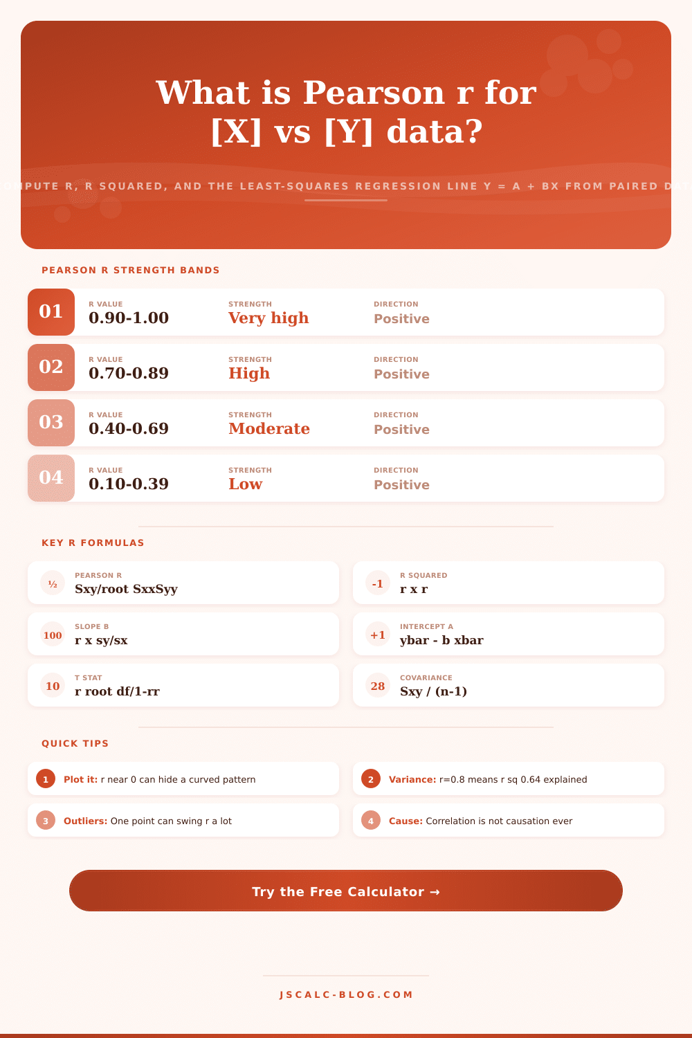
📊Correlation Strength Bands
| Absolute r | Strength | What It Means for a Scatter Plot |
|---|---|---|
| 0.90 to 1.00 | Very strong | Points hug the line tightly |
| 0.70 to 0.89 | Strong | Clear linear trend, little scatter |
| 0.40 to 0.69 | Moderate | Trend visible but noticeable spread |
| 0.10 to 0.39 | Weak | Slight tilt, lots of scatter |
| 0.00 to 0.09 | Negligible | Essentially a flat cloud |
📏Critical r Values by Sample Size
| n pairs | df = n - 2 | Critical r at 0.10 | Critical r at 0.05 | Critical r at 0.01 |
|---|---|---|---|---|
| 5 | 3 | 0.805 | 0.878 | 0.959 |
| 6 | 4 | 0.729 | 0.811 | 0.917 |
| 8 | 6 | 0.621 | 0.707 | 0.834 |
| 10 | 8 | 0.549 | 0.632 | 0.765 |
| 15 | 13 | 0.441 | 0.514 | 0.641 |
| 20 | 18 | 0.378 | 0.444 | 0.561 |
| 30 | 28 | 0.306 | 0.361 | 0.463 |
| 50 | 48 | 0.235 | 0.279 | 0.361 |
| 100 | 98 | 0.165 | 0.197 | 0.256 |
📈r Versus r Squared Interpretation
| Pearson r | r squared | Variance Explained | Practical Read |
|---|---|---|---|
| 1.00 | 1.00 | 100% | Perfect straight line |
| 0.90 | 0.81 | 81% | Very strong fit |
| 0.80 | 0.64 | 64% | Strong, one third unexplained |
| 0.70 | 0.49 | 49% | About half explained |
| 0.50 | 0.25 | 25% | Only a quarter explained |
| 0.30 | 0.09 | 9% | Weak, mostly noise |
| 0.10 | 0.01 | 1% | Almost nothing explained |
✅Pearson r Assumptions Checklist
| Assumption | Why It Matters | Quick Check |
|---|---|---|
| Linearity | r only measures straight-line fit | Look at the scatter plot |
| Paired numeric data | Each X needs one matching Y | Equal list lengths |
| Interval or ratio scale | Ranks need Spearman instead | Values are true measurements |
| No extreme outliers | Single points can distort r | Inspect min and max |
| Roughly bivariate normal | Needed for the t-test p value | Symmetric, no heavy skew |
| Independent observations | Repeated measures bias r | One row per subject |
🗃Sample Size Versus Critical r Comparison Grid
| n pairs | df | Crit r 0.10 | Crit r 0.05 | Crit r 0.01 | Min r for Strong |
|---|---|---|---|---|---|
| 5 | 3 | 0.805 | 0.878 | 0.959 | 0.70 |
| 7 | 5 | 0.669 | 0.754 | 0.874 | 0.70 |
| 9 | 7 | 0.582 | 0.666 | 0.798 | 0.70 |
| 12 | 10 | 0.497 | 0.576 | 0.708 | 0.70 |
| 16 | 14 | 0.426 | 0.497 | 0.623 | 0.70 |
| 25 | 23 | 0.337 | 0.396 | 0.505 | 0.70 |
| 40 | 38 | 0.264 | 0.312 | 0.403 | 0.70 |
| 60 | 58 | 0.214 | 0.254 | 0.330 | 0.70 |
| 80 | 78 | 0.185 | 0.220 | 0.286 | 0.70 |
| 120 | 118 | 0.151 | 0.179 | 0.234 | 0.70 |
⚙Formula Breakdown
💡Correlation Reading Tips
It’s easy to enter both sets of numbers in the two columns and see if there is any connection at all. Perhaps it’s the amount spent on advertising versus monthly revenue, or maybe it’s the number of hours studying versus the score on an exam. Whatever the connection may be… Does it exist? How strong is it?
That’s where the Linear Correlation Coefficient (r) Calculator comes in. Paste in your pairs of numbers and click calculate. You will get a precise answer to your question and a lot more. Several concepts appear, including standard deviation, covariance, and the least squares regression line. You will also see coefficient of determination r squared, Pearson r value, and a significance test. The hard math work is done for you while you can concentrate on interpreting what it all means to you personally.
Understanding the Linear Correlation Coefficient Calculator
Pearson r are a number between minus one and plus one. The higher it is, the more closely related two variables are on a straight line. This is why it is called Pearson’s Correlation Coefficient or Pearson r. Because of this it is a unitless quantity.
Near zero indicates there is no linear relationship, but does not necessarily mean there is no relationship. You might just have a perfectly U-shaped curve with an r close to zero because the trend reverse direction. This is where folks go wrong. If Pearson r is low then they think Y and X must be independent, when what might really be true is that Pearson r only measures straight line relationships. Plot your data first. If your points make a parabola, r will lead you astray despite how predictable Y are given X.
The math is also relatively straightforward, though it’s done rigorously. First, the calculator find the deviation from the mean for each variable. Then it squares these, adds them, divides by the square root of the product of the two squared sums, and finally rescales them. What this does is remove the units so you can judge how strong an association is between weight and height compared to, say, energy use and temperature.
The sign of r tell us the direction: One goes up; the other down. A positive number mean they go up together. Negative is when one goes down as the other goes up. Magnitude tells you strength. Above 0.7 is generally regarded as strong; below 0.4 is weak.
If you square r you get something that is called r squared, and also known as coefficient of determination. It’s perhaps a more practical number for people trying to make decisions, since we can read it directly as a percentage. If your r is 0.8 then your r squared is 0.64, that means that sixty four percent of the variance in Y is attributable to X. Thirty six percent of it is either noise or caused by other things which you haven’t measured. This helps explain why modest correlations may be disappointing in practice. An r of 0.5 sounds pretty strong, but it actualy only accounts for twenty five percent of the variation. That leaves the rest unaccounted for.
It also plots a regression line through your data points. You can use that line, written y equals a plus bx, to make predictions. B is called the slope; it represents the change in Y per unit of X. A anchors the line where X equals zero. The calculator calculates these based off the same sums of squares that r relies on.
It also conducts a t test to determine whether your correlation is meaningful (statistically significant) or merely a result of having such a small sample. To achieve statistical significance with only five pairs of data, you would of to have an extremely high r. With a larger sample, weaker correlations grows statistically significant. That’s important because large datasets can have weak but real relationships, and tiny ones may contain strong relationships that are pure chance.
Do verify your input. Confirm that you have interval scaled, numeric data. R is sensitive to outliers, which will tug the line towards themselves and skew results. A single outlier can make a mild relationship appear to be much stronger or much weaker than it is. Fortunately, the calculator includes some other stats such as standard deviations and how variables change together that allow you to see this influence. Standard deviation maintains the units of measurement, which makes the result difficult to grasp, but demonstrates the actual variance in raw numbers prior to the standardizing process. Seeing the spread. And mean, gives you more context for the snugness or looseness of your cloud of data points.
Remember that correlation is not necessarily causation. There may be an increase in ice-cream sales and drownings, but that doesn’t mean that ice-cream sales cause drownings. They’re both caused by the summer heat. Mathematically speaking, there is a connection as evidenced by the calculator, but you need to supply the domain expertise to make sense of it.
To help with this, it has some presets for common associations (such as GPA vs study time, height vs weight) so that you can test your familiarity with them before trying something yourself. When you input your own data, whether to confirm a scientific theory or validate a business hunch, the numbers will indicate how confident you should feel about a linear relationship between two things.
Finally, remember: always look at your data, you’ll see things a simple coefficient can’t. Test its significance so you’re sure it’s not just luck. Use r squared as a measure of how much it explains. And keep that mix of intuition and math. It turns raw data into real insight.