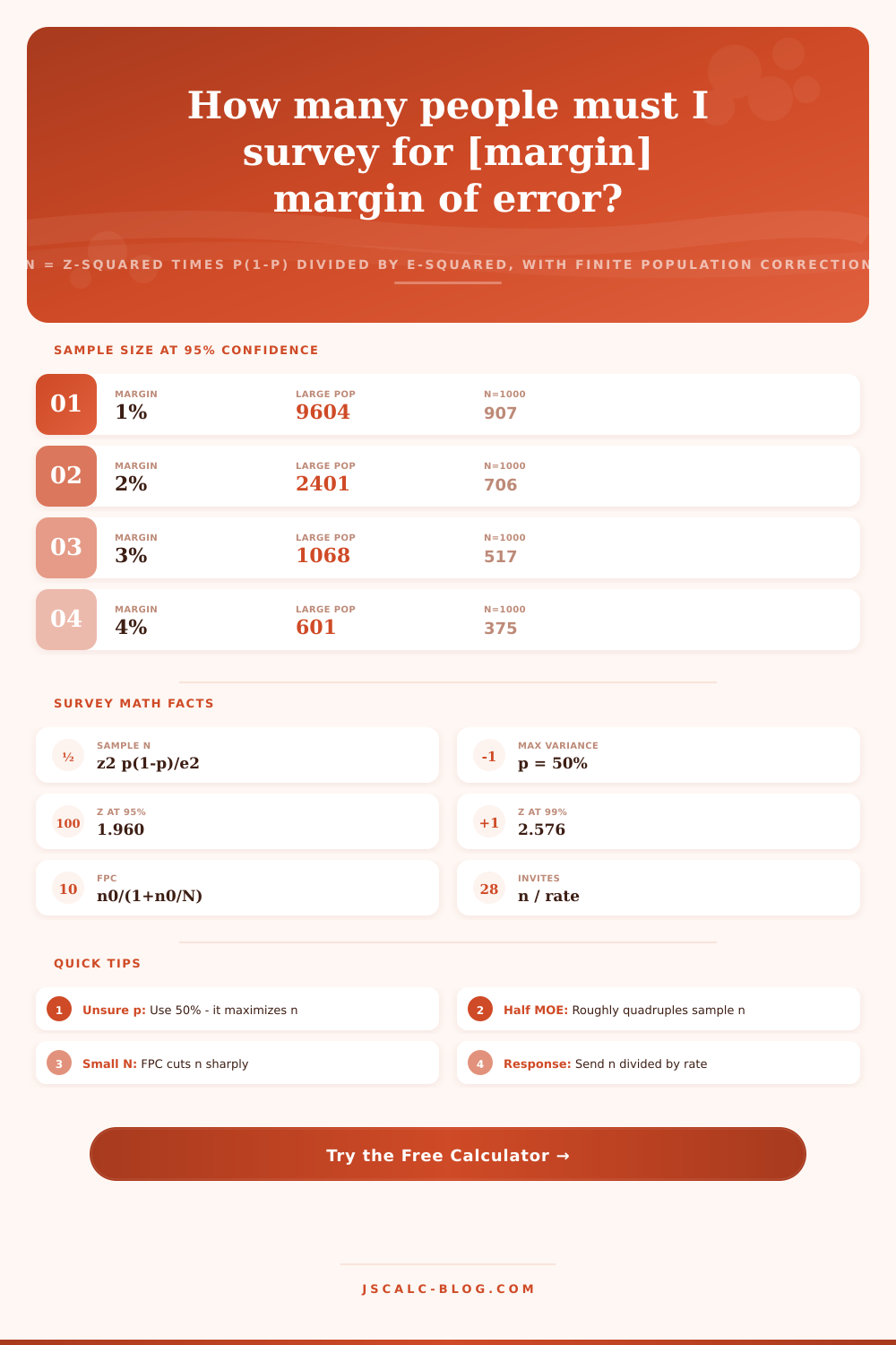
Sample Size for Survey Calculator
Work out how many completed responses your survey needs using n = z-squared times p(1-p) divided by e-squared, apply the finite population correction when you know the population size N, and turn the target into invitations to send from your expected response rate. You can also reverse the math to find the margin of error a fixed sample can actually deliver.
👥Choose a Mode
🎯Real Survey Presets
📝Survey Inputs
How sure you want to be the true value sits inside the margin.
Half-width of the confidence interval, in percentage points.
Share picking the key answer. Use 50% when unsure for max n.
Choose unlimited to skip the finite population correction.
Total people in the group you are studying.
Share of invitees who finish. Sets invitations to send.
Used in margin-of-error mode to reverse-solve e.
Controls rounding on the margin and rate figures.
🔢Formula Snapshot
📋Z Score by Confidence Level
| Confidence Level | Alpha (two tail) | Z Score Used | Typical Use |
|---|---|---|---|
| 80% | 0.20 | 1.2816 | Quick internal pulse |
| 85% | 0.15 | 1.4395 | Low-stakes screening |
| 90% | 0.10 | 1.6449 | Pilots and drafts |
| 95% | 0.05 | 1.9600 | Standard reporting |
| 98% | 0.02 | 2.3263 | High-stakes decisions |
| 99% | 0.01 | 2.5758 | Clinical and finance |
| 99.9% | 0.001 | 3.2905 | Safety-critical claims |
📊Sample Size at 95% Confidence (Large Population, p=50%)
| Margin of Error | Required n | Precision | Effort Level |
|---|---|---|---|
| +/- 1% | 9,604 | Very precise | Large budget |
| +/- 2% | 2,401 | Precise | Substantial |
| +/- 3% | 1,068 | News-poll grade | Moderate |
| +/- 4% | 601 | Solid | Reasonable |
| +/- 5% | 385 | Common default | Light |
| +/- 7% | 196 | Rough | Very light |
| +/- 10% | 97 | Directional only | Minimal |
📏How Population Size N Shrinks Required n (FPC, 95%, +/-5%)
| Population N | Uncorrected n0 | Corrected n | Percent of N |
|---|---|---|---|
| 100 | 385 | 80 | 80% |
| 500 | 385 | 218 | 44% |
| 1,000 | 385 | 278 | 28% |
| 2,000 | 385 | 323 | 16% |
| 5,000 | 385 | 357 | 7% |
| 10,000 | 385 | 370 | 4% |
| 50,000 | 385 | 382 | 1% |
| 100,000+ | 385 | 384 | Under 1% |
📧Response Rate Benchmarks by Channel
| Survey Channel | Typical Rate | To Get 385 n | Note |
|---|---|---|---|
| In-person intercept | 50 - 70% | ~640 asks | Highest yield |
| Phone / telephone | 10 - 20% | ~2,570 calls | Declining fast |
| Email invitation | 20 - 30% | ~1,285 sends | List quality matters |
| SMS / text | 15 - 25% | ~1,925 texts | Short surveys only |
| Web pop-up intercept | 2 - 5% | ~9,625 views | High traffic needed |
| Panel (paid) | 40 - 60% | ~770 invites | Fast but costs |
| Postal mail | 5 - 15% | ~3,850 letters | Slow turnaround |
🗃Required n by Confidence and Margin (p=50%, Large Population)
| Margin of Error | 80% Conf | 90% Conf | 95% Conf | 99% Conf |
|---|---|---|---|---|
| +/- 1% | 4,107 | 6,765 | 9,604 | 16,587 |
| +/- 2% | 1,027 | 1,692 | 2,401 | 4,147 |
| +/- 3% | 457 | 752 | 1,068 | 1,843 |
| +/- 4% | 257 | 423 | 601 | 1,037 |
| +/- 5% | 165 | 271 | 385 | 664 |
| +/- 7% | 84 | 139 | 196 | 339 |
| +/- 10% | 42 | 68 | 97 | 166 |
⚙Formula Breakdown
💡Survey Planning Tips
Before you start gathering results, decide how many answers you’ll need to reach. A simple rule of thumb is this: use standard formula for estimating a population proportion in sample size calculator to immediately see how many responses you’ll need. If you also have an idea of how large your entire group is (e.g., 1 million potential customers), then enter that and it will recalculate the sample size based on your actual total. Turning the statistic into a concrete number of responses you need. This ensures that you don’t copy and paste figures from existing research or guess at what’s appropriate; instead you can rely on the calculator to give you a number that reflects your desired precision and confidence level. Getting this wrong affects not only accuracy but also efficiency: over-sampling costs time; under-sampling costs money.
That’s the basic formula: $n_0 = (z^2 \times p \times (1-p)) / e^2$. Here, $e$ is your margin of error expressed as a decimal. $p$ is the proportion of a particular answer that you expect to see. Finally, $z$ is the z-score corresponding to your desired level of confidence. The normal distribution tell us what z-scores should be for certain levels of confidence. For example, at ninety-five percent confidence, we use a z-score of 1.96. Plugging those values into the above equation with a margin of error of 0.05 and an expected proportion of 0.5 gives approximately 385 respondents. That happens to be pretty common among professional polls; it’s used by default in many situations, so it tends to work out okay.
How to Choose the Right Sample Size
Because the variance term spikes at $p =.5$, the value of $p$ has a strong influence on the outcome. The product of 0.5 times 0.5 is 0.25, the maximum value for this product. Every other combination (e.g., 20 percent / 80 percent) yields a lower product, requiring a smaller sample. Entering 50 percent is the conservative play, since it ensures that you’ll always have enough people in your sample. You might be able to enter a different number if past studies indicate the actual proportion is likely closer to 20 percent; however, you shouldn’t do so unless evidence is compelling.
In practice we assume our population is effectively infinite, which is fine if you are polling at the national level but wasteful when polling smaller populations such as a town with two thousand residents or a company with five hundred employees. That’s where the finite population correction comes in: it divides your uncorrected sample size by something that takes into account the total size of the population $N$. For small populations (such as 500), this has dramatic effects, reducing 385 down to approximately 218. As $N$ rise into the tens of thousands, the correction becomes small, and pollsters can ignore it while still hitting close to their benchmark standards.
However, this still doesn’t tell you exactly how many invitations to send since not everyone will complete the survey. To figure out how many invitations to send, the calculator takes your target (385) and divides it by the response rate you expect. Assume 30 percent completion, and then you would invite about 1,284 (385/0.3). The channel hugely impacts the response rate. Online pop-ups can be as low as a few percent, whereas intercepts done in person is usually at least 50 percent or higher. Don’t let the “missing” hundreds of responses happen to you… Build the response rate into your plan upfront.
If you’ve got a dataset and have already gathered it, sometimes your sample size is set in stone: there’s just a thousand contacts on your list, and that’s all you can work with. Then the relevant question becomes: How accurate will my findings be with such a sample? That’s where the margin-of-error mode comes in, which rewrites the equation to solve for $e$. When applied to a large population and a sample size of one thousand respondents, a margin of error is approximately plus or minus 3.1 percent (at ninety-five percent confidence). This reverse-calculation serves as a necessary tool for making sense of data we’re given.
The denominator includes the margin of error e, which is why halving the margin of error quadruples the needed sample (that’s what reference tables illustrate; note that the margin of error is squared). For example, increasing the margin-of-error from plus or minus 5 percent to plus or minus 2.5 percent increases the necessary sample from 385 to approximately 1,537. Demanding a margin of plus or minus 1 percent increases it to 9,604.
In general, raising confidence levels will work the same way: Sensible survey design involves selecting the largest margin and loosest confidence that your decisions can truly sustain. Sound sampling is the difference between the numbers that mislead you and those that you can trust. You should of started with your constraints and let the math determine the rest.