Units of Production Depreciation Calculator
Calculate depreciation per unit, current period expense, accumulated depreciation, remaining units, and ending book value while enforcing the salvage value floor.
🎯Production asset presets
🔢Asset and production inputs
Uses meter-backed operating hours.
Examples: hours, miles, cases, impressions, cycles, tons.
Include purchase price and capitalized setup needed to use the asset.
The calculator will not depreciate book value below this floor.
Use total expected production over the asset's useful life.
Prior production units recognized before this period.
Current month, quarter, job, or reporting period output.
Used for straight-line comparison and remaining-year estimate.
Controls the comparison schedule, not the core units formula.
Per-unit rates always show enough decimals for small-unit assets.
Formula breakdown
📌Selected asset reference grid
📊Current period comparison grid
📅Six-period depreciation schedule
| Period | Units | Depreciation | Accumulated | Ending book value |
|---|
🔍Actual units sensitivity table
| Scenario | Period units | Period depreciation | Ending book value | Floor status |
|---|
⚖Depreciation method comparison table
| Method | Current period formula | Current depreciation | Best fit | Caution |
|---|
📘Production basis quick reference
| Asset group | Common unit | Good evidence | Useful estimate check |
|---|---|---|---|
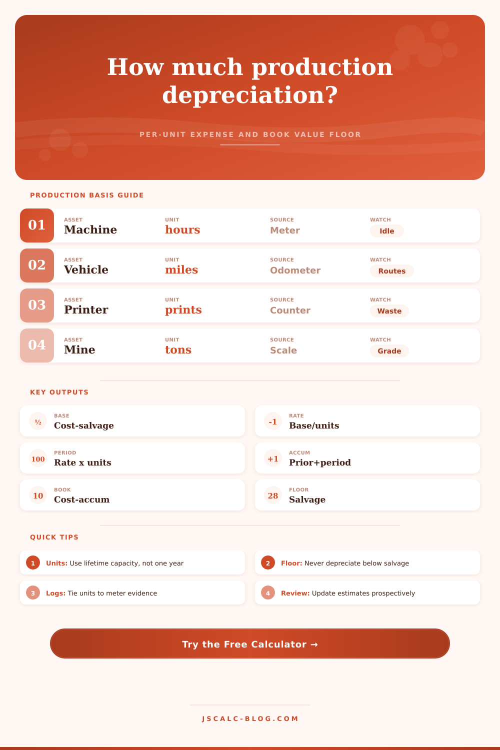
| Manufacturing machine | Operating hours | Machine meter or PLC log | Capacity plan, maintenance history |
| Delivery vehicle | Miles or km | Odometer and route log | Fleet policy and route density |
| Production line | Finished units | Batch close report | Rated throughput and downtime |
| Print equipment | Impressions | Counter reads | Duty cycle and waste rate |
| Tooling or mold | Cycles or shots | Press counter | Material abrasiveness and refurb plan |
| Extraction asset | Tons or barrels | Scale tickets or production report | Reserve estimate and depletion plan |
| Energy equipment | Runtime hours | SCADA or hour meter | Capacity factor and outage schedule |
| Lab equipment | Scans or cycles | Instrument counter | Calibration interval and rated cycles |
🧮Formula and floor rules
| Step | Formula | What it means | Calculator safeguard |
|---|---|---|---|
| Depreciable base | Asset cost - salvage value | Maximum amount to depreciate | Salvage cannot exceed cost |
| Per-unit rate | Base / estimated total units | Fixed depreciation per output unit | Total units must be positive |
| Period expense | Rate x actual units | Expense tied to this period's production | Caps at remaining depreciable base |
| Accumulated depreciation | Prior depreciation + period expense | Total depreciation recognized to date | Never exceeds depreciable base |
| Book value floor | Cost - accumulated depreciation | Net carrying value after depreciation | Never below salvage value |
💡Production depreciation tips
Typically, depreciation accounts is based on time. Your assets depreciate at a consistent rate each year regardless of how often they are used. Straight-line depreciation treats time as the primary driver of loss, assuming that your asset loses an even amount of value per year regardless of how much it’s being used.
Units of production depreciation flips that thinking around. According to its logic, the asset lose value only when it’s used, not when time passes. You turn on your CNC machine and run it for ten thousand hours during the year. You then turn it off for two years. According to units of production depreciation, the cost should of reflect what happened: you paid for usage. That makes units of production depreciation more aligned with physical reality.
How Units of Production Depreciation Works
And that’s why, after plugging in your assets’ details into the calculator, we’ll do the math for you. It’s pretty straightforward: Depreciation = (asset price, salvage value) / expected lifetime units. Divide the depreciable base by how many units you anticipate producing during the lifetime of the asset. That yields a constant per-unit expense. Multiply that constant by the number of units you actualy produced during some time frame; that produces your depreciation expense for that period.
Easy enough, except how do you estimate those total units for the whole life of the asset? Guess too high, and your book value will be creeping down. Guess more low, and you’ll write off more than the underlying asset was really worth. The tool has a safety feature to prevent that. Once the book value reaches what you think the asset would sell for as scrap, the tool won’t keep on losing value. In other words, it floors at the salvage value.
Most folks gets tripped up in the choice of unit of measure. What unit captures wear (and only wear? If it’s a delivery van), miles is good: you stress the engine at every mile. If it’s a printing press, then impressions are right since each one stresses the machine. For a mine conveyor, maybe it’s operating hours. However, if the load varies widely, a better proxy will be tons moved. The table on the page lists some common pairings across asset classes; it will help you make a reasoned choice rather than a random one. Your goal is to pick the unit that moves as the metal wears down.
In the real world things don’t come in neat curves. Unexpected breakdowns occur. Maintenance shutdowns happen. Production spikes occurs. Your actual units won’t be what you predicted. And when that occurs? Do you go back and change history? No. You adjust going forward. Realize you’re only getting twenty thousand hours out of this machine instead of thirty? Then figure out how much of the depreciable base is left to depreciate on remaining capacity. That keeps your books clean while avoiding any awkward prior-period adjustment. It requires a slight admin lift but offers big gains for preserving an accurate profit margin on future periods.
When you’re producing at a steady rate, this approach naturaly smooths out the volatility in your net income. On the one hand, if you fall into a slow period (due to market conditions); your depreciation expense falls as well so it protects cash flow reporting. On the other hand, when it’s a boom year, higher revenues is matched by higher expenses, which can reduce your tax liability on those critical days when it realy counts. The matching principle is a powerful thing. It connects the cost of the tool to the revenue it produces.
At the end, units of production depreciation requires honest accounting. It does not assume an asset has worn out just because time passed. It tracks what actualy happened. This is whether you’re measuring tons produced by a mining rig, or shots produced by an injection mold. What matter is the same: make the expense reflect the use. Use the calculator; it’s easy. But make sure the input data accurately reflects how the tool is actually used in the real world. If you do so, all else follows.