Sum of Squares Calculator
Calculate total sum of squares SST = sum((xi - mean)2), raw sum squares = sum(xi2), corrected SS, and between or within group ANOVA components.
Load a data pattern, then adjust the values, groups, units, and decimal precision.
Enter at least two observations to calculate sum of squares.
Group mode calculates SSB, SSW, SST, ANOVA degrees freedom, and F ratio.
Displayed values round here; formulas use full precision internally.
Examples: scores, weights, yields, ratings, times, or measurements.
Leave blank for unitless data; squared results append ^2.
This highlights the related rows in the reference tables.
All valid observations are used; this only limits the displayed breakdown rows.
Separate values with commas, spaces, semicolons, tabs, or line breaks.
| Group | x value | x2 | x - grand mean | (x - mean)2 | Within group part |
|---|---|---|---|---|---|
| Enter data to see each observation contribution. | |||||
| Group | n | Group mean | Raw SS | Within SS | Between contribution |
|---|---|---|---|---|---|
| Group details appear after calculation. | |||||
| Measure | Formula | Current value | Degrees freedom | Use |
|---|---|---|---|---|
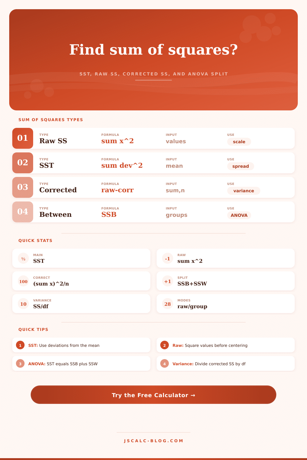
| Total SS (SST) | sum((xi - mean)2) | 0 | n - 1 | Spread around the grand mean |
| Raw sum squares | sum(xi2) | 0 | none | Uncentered square total |
| Correction term | (sum x)2 / n | 0 | none | Amount removed by centering |
| Corrected SS | sum(xi2) - (sum x)2/n | 0 | n - 1 | Variance numerator |
| Between SS | sum(ng(meang - mean)2) | 0 | g - 1 | Group mean differences |
| Within SS | sum sum((xig - meang)2) | 0 | n - g | Residual spread inside groups |
| Source | SS | df | Mean square | Current context | Variance link |
|---|---|---|---|---|---|
| Between groups | 0 | 0 | 0 | Explained by group means | MSB = SSB / df |
| Within groups | 0 | 0 | 0 | Residual within groups | MSW = SSW / df |
| Total | 0 | 0 | 0 | SST = SSB + SSW | Total variance = SST / df |
| F ratio | 0 | between / within | MSB / MSW | Needs 2+ groups | ANOVA signal check |
| Eta squared | 0 | proportion | SSB / SST | Share explained by groups | Effect size cue |
| Sample variance | 0 | n - 1 | SST / (n - 1) | For one combined sample | variance calculator |
If you learned statistics, you probably did so using pencil-and-paper calculations. You entered values, you added them, you squared them, you checked if you dropped any decimal. It’s boring. It seem more like error-accounting than anything else.
And in many ways, the sum of squares serve as the basis for variance, ANOVA, and regression. But we tend to view this as a rote computation. It is a way to calculate the spread of our data that is actualy quite meaningful. What you’re doing is trying to capture how far off of what you expected your data is. That distance, that spread, that’s the story. Math is just person telling the tale.
What Is the Sum of Squares?
After pasting in your group data or raw scores, the calculator takes over the math. No more arithmetic mistakes due to being bored and/or tired. At the same time, it calculate the corrected sum of squares, the raw sum of squares, and the total sum of squares. These three value represent the same numbers but in slightly different ways.
The total sum of squares describe how widely the data points are distributed around grand mean. The raw sum of squares is the sum of each individual value squared. While this has uses in other algebraic shortcuts, it’s not particularly informative alone regarding variability. The corrected sum of squares, however, is what you want for calculating variance. It correct for the mean. In doing so, it centers the data, allowing you to view actual distribution.
The distinction between these measures is more important than knowing the formulae themselves. Why are the test results different? If all students got roughly the same score, then the total sum of squares will be small. If they did very differently, it’ be large. Understanding why that’s true is important. Is there some reason (teaching style, etc.) that accounts for those difference? Or is it just randomness?
That’s where the breakdown between the within- and between-group sums of squares comes in. The calculator does this automatically but you should of understand what it means. The between-group sum of squares tell you how much each individual group differ from the mean of all groups. The within-group sum of of squares tells you how much each person differs from his/her group average.
That’s where the split comes in with ANOVA. It’s asking: Are the differences among groups greater than the difference within each group? If the between value is large relative to the within value, then your groups are distinct. If it’s similar, then the group labels don’t matter much. That ratio reflect how strong an effect the experimental conditions may has had on you.
A lot of people gets confused about degrees of freedom. They think that they’re just some abstract math term. No, they aren’t. They reflect the independent information remaining after accounting for things such as the mean. Dividing by those degrees of freedom give us the mean square. This allows us to fairly compare even though our samples might differ in size.
One common error people make is confusing the correction term. The correction factor is simply (sum of squared values)/(number of observations). To obtain the corrected sum of squares, you subtract this value from the uncorrected sum of squares. This will cause your estimate of variance to be inflated. What’s more, your results will be invalid.
Note that this identity appears in the reference table in the tool. You can use this to confirm that the total matches the sum of the within and between terms. Do not neglect this sanity check.
This can be applied in practice. For example, you can evaluate plant growth, clinical outcomes, or production lines. In each case, the logic is the same. Did the change you introduced cause the change you observed? And did you introduce a change? If so, then what’s the relationship between these two changes?
The sum of squares captures this relationship in a good way, standardized and robust. It strips away the units and measures the magnitude of deviation. That’s why it’s widely used. It works for weights, times, ratings, or any numeric data.
So, easy? Yes. Advanced modeling isn’t required to begin understanding variation. Square the deviations. Sum. The calculator does the math. But you supply the meaning. What’s being measured? What’s the grouping? How do you make sense of the numbers? They’re your signal, but they also contain noise. Interpret that.
Analyze sensor data or test results. Same idea. Strip out the signal from the background static. It’s tiny, but significant. Measure the spread and you know the structure. And that helps clarify things. It’s worth the work.