At Least One Event Probability Calculator
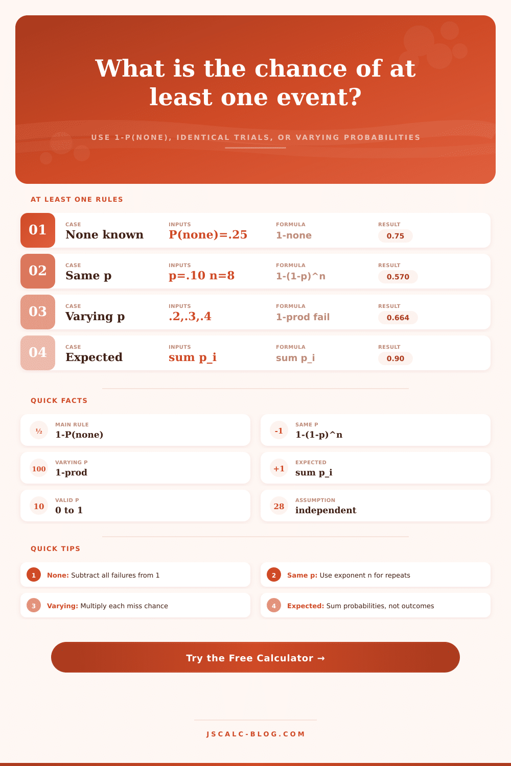
Find the chance that one or more independent events happen, using identical trial probability, varying probabilities, or a known none probability.
🎯At Least One Presets
⚙Probability Inputs
Choose the formula that matches your available inputs.
The same format is used for all probability fields.
For identical trials: p in 1 - (1 - p)^n.
Use a whole number of repeated chances.
Used in the interpretation and table labels.
Internal calculations keep full precision.
Calculated from 10 identical independent trials at 12% each.
🧮Current Probability Snapshot
📐At Least One Formula Table
| Situation | Formula | Use When | Expected Hits | Assumption |
|---|---|---|---|---|
| Known none probability | P(at least one) = 1 - P(none) | You already know the all-fail chance | Not implied by none alone | None probability is valid |
| Identical independent trials | 1 - (1 - p)^n | Same event chance repeats n times | n x p | Trials are independent |
| Varying independent probabilities | 1 - product(1 - p_i) | Each attempt has its own p | sum p_i | Events are independent |
| Rare small probabilities | 1 - product misses | Low p but many attempts | Often near total risk | No shared cause omitted |
| Impossible overlap check | P(at least one) must be 0 to 1 | Auditing entered probabilities | Cannot exceed trial count | Inputs stay in range |
📊Identical Trial Quick Table
| Per-Trial p | 5 Trials | 10 Trials | 20 Trials | 50 Trials | Expected in 10 |
|---|---|---|---|---|---|
| 1% | 4.90% | 9.56% | 18.21% | 39.50% | 0.10 |
| 2% | 9.61% | 18.29% | 33.24% | 63.58% | 0.20 |
| 5% | 22.62% | 40.13% | 64.15% | 92.31% | 0.50 |
| 10% | 40.95% | 65.13% | 87.84% | 99.48% | 1.00 |
| 20% | 67.23% | 89.26% | 98.85% | 99.999% | 2.00 |
| 50% | 96.88% | 99.90% | 99.9999% | ~100% | 5.00 |
🗂Common Scenario Comparison
| Scenario | Probability Pattern | At Least One Formula | Expected Hits | Watch For |
|---|---|---|---|---|
| Sales outreach | Same close rate per lead | 1 - (1 - p)^n | n x p | Lead quality may vary |
| Quality defects | Defect chance per item | 1 - (1 - p)^n | items x p | Batch defects can correlate |
| Mixed campaign | Different channel rates | 1 - product(1 - p_i) | sum p_i | Duplicate audiences |
| System uptime | Independent component failures | 1 - product(1 - p_i) | sum failure p_i | Shared power or network risk |
| Game attempts | Fixed odds each try | 1 - (1 - p)^n | tries x p | Assume fair repeated odds |
| Clinical endpoint | Risk per participant or period | 1 - product misses | sum endpoint risks | Do not infer causality |
| Known all-clear rate | Only P(none) available | 1 - P(none) | Not enough information | No count breakdown |
📋Method Breakdown
💡Practical Probability Tips
Let’s say there’s a 12% probability of a client replying to your cold email. You can fire off ten emails which means there’s an expected value of 1.2 replies. You may look at that and think: “hmm, I don’t like my chances here.” Maybe ten percent is too low? Maybe I only have a twelve percent shot of getting something? Your gut says no, but that’s typically incorrect. Because it doesn’t account for how probabilities compound with repeated effort. In fact, you’ve got about a 72% chance of hearing back from someone… which is a huge difference than what your gut thinks.
And this applies in everything from engineering to sales; it’s the idea behind what we call at least one probability. The key trick here is what I call the complement rule: You don’t multiply out the chances of getting exactly one success, or two, or ten; you calculate the chance of total failure (which would be missing every time) and subtract it from 1. If there’s an 88% chance of someone ignoring any given email, then ignoring all 10 emails is that 88% raised to the 10th power, which is a lot lower than 88%.
Why Trying Many Times Helps You Succeed
The point of taking many shots is that volume can trump perfection when you’re in an uncertain environment. You don’t have to get a better conversion rate; you just has to take enough independent shots. If you’ve got a regular old repeat situation, just plug it into the top calculator and let it do the math.
But life doesn’t always fit so neatly in that box. More likely than not, different channels is going to have different probabilities. Maybe one server component is on its last legs; maybe another’s rock solid. Maybe one marketing campaign will go real well; maybe another won’t. If you’re dealing with situations like these, where there’s no “multiply this many times” to your probability, because every try counts separately. Then you need a tool which can take account of each individual attempt. The tool does this by allowing you to list separate probabilities for each event and then multiplying the miss chance of each to give you total risk of all failing.
It’s a subtle shift in thinking, but it helps avoid being too careless about risks. Another measure that often confuses people is called expected hits. That’s the total of every probability. So for instance in our email case, we have ten trials with a twelve percent chance of reply. Our expected value is 1.2 replies. Now let me be clear: This doesn’t mean there’s a one point two chances that you’ll recieve one email. It means that on average, across a hundred such campaigns, you’d expect to receive one point two replies.
At least one probability is the likelihood your campaign immediately succeeds; expected value is the long-run volume. The two are related but distinct. Muddling the two can lead to wrong use of resources. You may look at an expected value > 1 and say “I’m gonna hit it!,” but remember that there’s still a meaningful chance that you’ll get nothing back.
The math relies on a silent assumption: independence. It assumes each event doesn’t affect future events. A server error that makes your email bounce isn’t an independent failure; it’s correlated with other bounces. Three servers going down during a power outage? Their probability of failure are related; it’s not independent. And in both examples, the typical calculation overestimates how safe you’ll be. Are the events really unrelated? If there’s some common thread connecting them, something that could fail, like a single point of failure, then the math fall apart. Most folks skip past that part when they copy-paste the formula.
If you look at the table on the page, it’s easy enough to see that the cumulative risk increases with each trial. If there are lots of opportunities, even a small probability of something going wrong dominates: one percent doesn’t sound like much, but after fifty tries, it means almost a 40% chance of a failure somewhere along the line. The graph curves up. That’s not intuitive. Probability builds up. Most of us live life thinking in straight lines. Learning about this curve shifts your perspective when planning around risk. It’s no longer “How likely is this one thing?”, it’s “how many times am I willing to give this one thing the opportunity to occur?”
But at its heart, it’s a question of using clarity to manage uncertainty. If you’re planning a sales sprint, or if you’re auditing a software system, it is key to understand the chance of any single thing happening versus the total number of things that might happen. It allows you to be properly skeptical of low probability outcomes without denying that total exposure will eventually lead to some sort of result. The math doesn’t make luck more likely, but it makes the nature of your risk clear. And once you know what your risk looks like, you can make better bets… even if they aren’t great ones. You should of seen this coming.