Sample Standard Deviation Calculator
Compute the sample standard deviation s using the n–1 Bessel correction, plus sample variance, mean, standard error of the mean, and coefficient of variation, with a full deviation table and a population comparison.
📊Real Data-Set Presets
📝Sample Data & Options
Enter a sample drawn from a larger population. At least 2 numeric values are required for the n–1 divisor.
🔢Formula Snapshot
📈Per-Value Deviation Table
| # | Value x | x – x̄ | (x – x̄)² |
|---|---|---|---|
| Enter sample values above to build the deviation table. | |||
| Sum of squared deviations (SS) | 0 | ||
📋Descriptive Summary
| Statistic | Symbol | Formula | Value |
|---|---|---|---|
| The descriptive summary appears after calculation. | |||
⚖Sample vs Population
| Measure | Sample (n–1) | Population (n) | Difference |
|---|---|---|---|
| The sample versus population comparison appears after calculation. | |||
🧮Why n–1? The Bessel Correction
| Sample n | Divisor n–1 | SS | Sample s² | Population σ² | Bias factor n/(n–1) |
|---|---|---|---|---|---|
| The Bessel correction grid appears after calculation. | |||||
⚙Full Formula Breakdown
📐Sample vs Population Reference
| Question | Use Sample (n–1) | Use Population (n) |
|---|---|---|
| What is the data? | A subset drawn from a larger group | Every member of the group |
| Symbol for SD | s | σ (sigma) |
| Divisor | n – 1 | n |
| Goal | Estimate the unknown population spread | Describe the known group exactly |
| Typical use | Surveys, experiments, quality samples | Census, full class, entire batch |
| Relative size | Always larger (bias-corrected) | Always smaller |
| Spreadsheet | STDEV.S / STDEV | STDEV.P / STDEVP |
💡Practical Sample SD Tips
We think standard deviation is just a measure of how spread out a set of numbers are and we are only partially right. What’s tricky about it is picking the proper divisor to give us an answer that shows wider picture. We’re sampling, such as when we take ten test scores or sample of 50 lab results. We don’t have entire population. Instead, we approximate it. If our approximation has improper mathematical divisor, then we’re going to come up short every time.
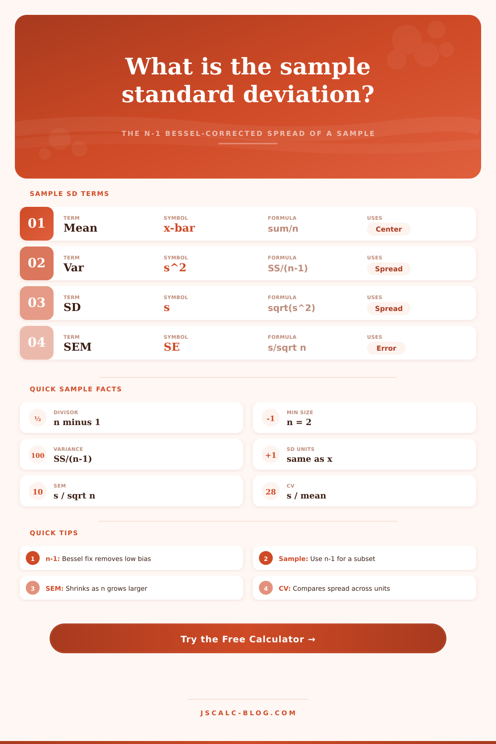
It’s one of those mistakes people make, they replaces a statistical adjustment with basic math. This is where Bessel correction comes into play. The calculator above takes Bessel correction into account and does the division by n, 1 instead. Why? Because there’s an issue with our data, it’s biased. Your individual data points forms a mean, which is located somewhere within your data set. However, those same data points is measured relative to themselves (their own center), making them look more tightly clustered compared to how they’d look when measured against the true center of the whole population. So dividing by a lower number correct for that false proximity, leaving you with an unbiased estimate of spread.
Why We Use n-1 for Sample Data
For instance, you might be analyzing quality control data across a manufacturing batch. Underestimating variance will make the process appear more stable then it actualy is. This is dangerous. You can enter your own set of numbers into the tool and then compare what the corrected results are relative to just doing a raw population calculation. The deviation table builds out row by row so you can see how much each individual value contribute to sum of squares. This helps make variance easy to see. It’s much simpler to wrap your head around seeing difference squared.
You can get a better view of what is happening with your data through related metrics. For example, a metric like the standard error of the mean tells you how accurately you’ve measured average. As your sample size grows this error shrinks. Where many analyses goes wrong is that individuals mistake wide spread for low confidence in the average. They’re not the same thing. Wide spread indicates that there’s a large distance between two adult-sized sofa, but a small standard error indicates high certainty on where the middle line sits (even though the other points around it may differ significantly).
Which formula do you apply? The answer is: it depends on context. With a full population, like a complete batch of products or all records in a census database, you’d divide by n. No guesswork there. But most business analytics, survey research, and other types of research is based off samples. They’re not examining entire populations. That means you need the n minus 1 version. That’s because sampling means you’re not seeing everything; you’re making an educated guess.
If you’re comparing two sets of data that are on different scales or even use different units, that’s where the coefficient of variation can comes into play. For example, does a standard deviation of five matter more if you’re talking about your weight in kilograms versus your height in centimeters? The coefficient strips out those units and shows a comparison between spread-to-mean as a ratio. That lets you also compare data of all sorts without having to worry about diffrent units.
Instead of complicated calculations, statistics is about being honest with what we represent. The sample isn’t complete. We admit as much in the n minus 1 fix. Then we adjust for it and we end up with something we could of rely on. The math does the work. But we understand why the math does the thing, and that’s where the insight comes. But we understand why the math does the thing, and that’s where the insight arrives.
Next time you see the final numbers, remember they are estimates. They are an approximation of what exists outside our collected data. That realization makes even a simple calculation a valuble way of understanding the world around us.