Residual Calculator
Calculate residuals from observed and fitted values, then inspect standardized residuals, studentized approximations, SSE, RMSE, leverage screens, and row-level diagnostic flags.
🎯Residual Presets
🧮Observed and Fitted Inputs
Use one case per line. Leverage is optional; blank leverage uses the default h below. Residual e = y - yhat.
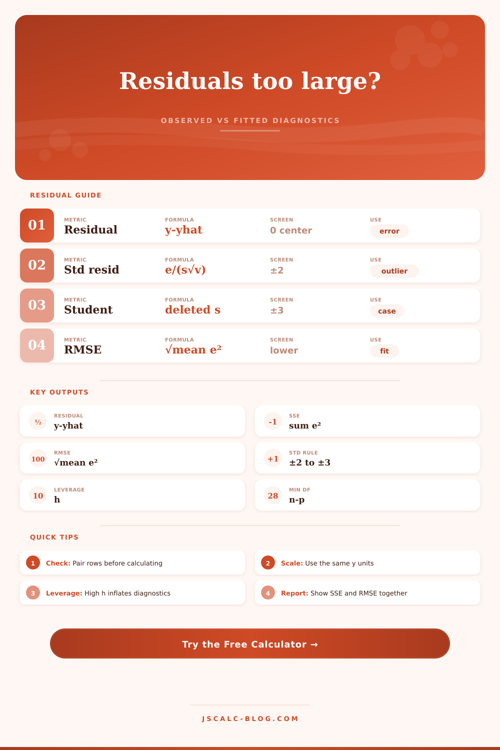
Standardized residuals use e / (s x sqrt(1 - h)).
Include the intercept. Regression residual standard error uses df = n - p.
Used only when the scale mode is fixed.
Applies to rows without a third numeric value.
External uses s_i from the case-deletion approximation when df allows it.
The row table flags standardized or studentized values beyond this cutoff.
📋Diagnostic Snapshot Grid
🔍Residual Breakdown Tables
Case-level residual table
Model error summary table
Diagnostic threshold table
Preset scenario grid
| Preset | Rows | Typical field | Leverage use | Scale mode | Diagnostic focus |
|---|---|---|---|---|---|
| Exam Score Model | 12 | Education | moderate h | SSE / df | missed students |
| Store Sales Forecast | 14 | Retail | mixed h | SSE / df | forecast misses |
| Clinical Recovery Scores | 10 | Health study | case h | fixed s | case review |
| Sensor Calibration Run | 12 | Lab quality | low h | RMSE | drift signs |
| Delivery ETA Model | 16 | Logistics | route h | SSE / df | late routes |
| Building Load Forecast | 12 | Energy | weather h | SSE / df | peak load |
| Home Appraisal Model | 10 | Housing | high h | fixed s | valuation error |
| Holdout Drift Check | 15 | Validation | default h | RMSE | drift flags |
| Production Yield Model | 12 | Manufacturing | batch h | SSE / df | yield misses |
📐Formula Reference
💡Residual Diagnostic Tips
The difference between what actualy happened and what you predicted: those is called residuals. So if you predicted exam scores or store sales using a regression model, then your fitted values represent story you told yourself. Your residuals test that story against reality.
Most of us will see our R-squared value and feel confident. That is a mistake. R-squared tell you how much variance you explained. Your residuals tell you how you failed. Understanding that failure is where we learn.
How to Read Model Errors
But don’t ignore those errors, as the patterns they expose would of been masked in your summary statistics. Your model could generally do pretty well yet misfire wildly for certain subgroups. Maybe it overestimate low scores and underestimate high ones. Or it could perform excellently during the week, but fall apart on weekends. Those aren’t average error. They’re structural weakness.
To compute studentized and standardized residuals for yourself, use calculator above. That way you’ll avoid manual division errors leaving more time to interpret what’s going on.
The primary instrument is standardized residuals. This simply divide your raw error by an estimate of its standard deviation (corrected for influence). Leverage measure how far an observation’s predictor values is from the rest of data. An extreme leverage point pull the regression line toward itself. When such an extreme leverage point have a big residual, it becomes an influential outlier that skews your model. The standardized residual bigger than two or three spots it. That’s arbitrary but helpful. It alert you to the rows needing your attention.
Beyond that, there’s studentized residuals, which estimate error scale while removing the given observation. Outlier can’t hide under the appearance of adding extra variability into the whole set. Instead, it give you a clearer picture as to whether one point truly sticks out. If you’re analyzing sensor calibration data or clinical recovery scores, that difference is significant. You cannot allow an extreme example to hide how extreme it is and make the other data points look noisier than they are.
The total error is what’s given by Sum of Squared Errors and Root Mean Square Error. Total squared deviation is also called SSE. It increases as sample size does, which makes it less useful on its own. But RMSE is better because it converts back in the original units of your outcome variable. If you’re predicting housing prices in dollars, RMSE will tell you how much the typical prediction is off in terms of dollars. But RMSE is also sensitive to large errors. Even though most predictions may be close, a few really big misses can spike this number. So you need both aggregate metric and the row-level diagnostics.
Many people miss the leverage check. Many people think that every data point are created the same. It’s not. Some points have disproportional power. We call these high-leverage points. These is the ones you mustn’t ignore or else you build a model that describes the outliers instead of the trend.
On the page there’s a table that outlines common residual and leverage thresholds, along with corresponding screens. This provide a fast heuristic: what to flag. Think of it like a flag, not a verdict. Investigate a flagged row instead of deleting it automatically. Maybe it’s a data entry mistake. Maybe it’s a new market segment. Context alone will tell you what.
There’s no need to get rid of residuals. There will always be residuals. There is a need to make residuals random. Any pattern in your residuals mean there’s something wrong with your model. You’re missing a variable. You need a different functional form. Or you need to admit that some things are inherently unpredictable.
Boring residual = good residual. It is a random scatter without any clear structure. That’s what a robust model looks like. The fact that the errors appear random means you’ve captured the signal and left the noise alone. It’s the best you can hope for.