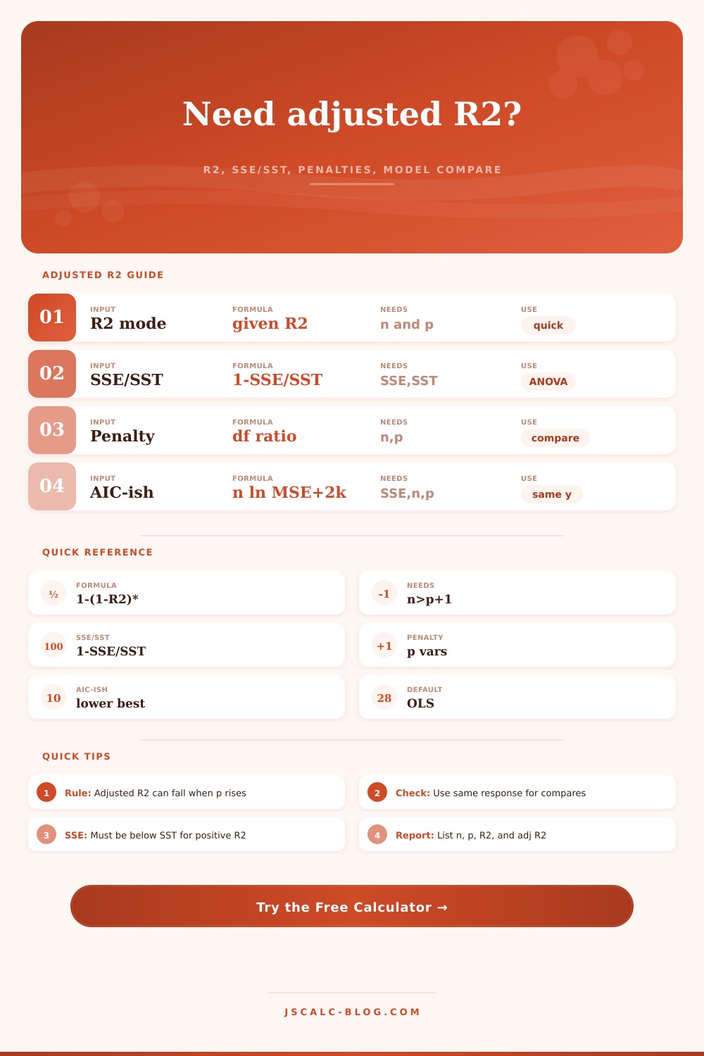
Adjusted R-Squared Calculator
Calculate adjusted R² from either a reported R² or sums of squares. Enter observations and predictor count, then inspect the degrees-of-freedom penalty, SSE/SST conversion, formula substitution, and optional AIC-like comparison for models fit to the same response data.
📌Model Presets
🧮Adjusted R² Inputs
SSE/SST mode computes R² = 1 - SSE / SST first.
The formulas here assume an intercept model and predictor count p.
Enter decimal R², such as 0.742. Values can be negative for unusual no-intercept reports.
Residual sum of squares. Used in SSE/SST mode and AIC-like comparison.
Total corrected sum of squares around the response mean.
Adjusted R² requires residual degrees of freedom n - p - 1.
Count slope terms, not the intercept. Indicator columns count as predictors.
Use label=Name, r2=0.70, p=4 or label=Name, sse=230, sst=800, p=4. AIC-like comparison uses n ln(SSE/n) + 2k only when SSE is available or derivable from shared SST.
📋Model Summary Grid
🔍Calculation Tables
Current model calculation
Reference comparison
Adjusted R² interpretation bands
| Situation | Adjusted R² behavior | What it suggests | Next check | Reporting note |
|---|---|---|---|---|
| R² rises, adjusted R² falls | Penalty exceeds new fit | Added predictors may be noise | Residual plots and validation | Prefer simpler model unless theory requires terms |
| Both rise | Fit gain beats penalty | New terms may help | Compare out-of-sample error | Report n and p with both R² values |
| Small n, high p | Large downward adjustment | Degrees of freedom are thin | Reduce terms or collect more data | State residual df clearly |
| Negative adjusted R² | Model underperforms mean baseline | Predictors explain little after penalty | Check specification and data quality | Negative values are possible |
| Near raw R² | Penalty is modest | n is large relative to p | Use validation for final choice | Adjusted R² is still in-sample |
AIC-like comparison rules
| Item | Formula used here | Required inputs | Valid comparison | Important limit |
|---|---|---|---|---|
| SSE path | score = n ln(SSE / n) + 2k | SSE, n, p | Same response values and same n | Lower is better within this set only |
| Parameter count | k = p + 1 | Predictor count p | Intercept linear models | Error-variance constants are omitted |
| Delta | current score - reference score | Two comparable scores | Negative favors current model | Do not compare different response scales |
| R² direct path | No absolute SSE | R², n, p only | Adjusted R² only | AIC-like score is hidden without SSE |
📐Formula Breakdown
💡Tips
So now you’ve got one more variable in your model. And the R-squared go up. This looks good. You’re explaining more of the dataset! That’s great! But the adjusted R-squared can goes down.
When that happens, it turns your exercise into not just arithmetic but also a debate about tradeoffs. Why? Because the raw R-squared is an over-optimistic metric. Adding predictors increases its value, including when they are predictors of noise. The metric does not penalize complexity.
What Is Adjusted R-Squared and Why It Matters
If you want to build a real-world model, that makes the raw R-squared a risky compass. The adjusted version correct this by punishing each new predictor you include in your equation. That’s just one way to think about it: a complexity tax. Add columns to your data set. But only get credit if they’re adding big value to the fit.
The calculator above does that math for you. It takes degrees of freedom out of the equation, and lets you spend more time thinking about how the model fits together. Input the number of rows in your sample, the number of predictor variables, and your existing sum of squares (or R-squared). Then let it perform the subtraction. Let it remove the illusion of perfection. Let it show you what remains once penalty is applied.
It’s a tiny calculation, but it shifts story of your findings. The penalty are driven by the number of predictors relative to the number of observations. If you have a massive dataset with thousands of rows and only five variables, the penalty is negligible. You’ll be able to safely ignore distinction between the raw and the adjusted score.
As you scale up variables and down samples, however, the penalty grow larger. That’s when folks tend to get tripped up. They assume that R-squared is some sort of unchanging measure of truth. It isn’t. It’s a statistic which change according to amount of data you use for it.
The degrees of freedom shown in the calculator, those are the residual degrees of freedom, remind us that we must maintain sufficient data points to justify our estimation of parameters. The danger of adding too many variables is overfitting, where you add predictors until your unadjusted R-squared appears respectable, then find the model doesn’t work when you apply it to new data.
The first line of defense against this is the adjusted R-squared itself. If you add a term, and its adjusted R-squared decreases, that’s a strong sign that this variable isn’t helpful at all. It’s increasing the complexity without adding more explanation. The table on the page explains this. It shows under what conditions result will be affected, such as when there is a large number of predictors or a small sample size.
In general, trust the drop more then the rise. What does all this mean in terms of how you’ll work with it? Suppose you’re creating a clinical outcome predictor (or a marketing mix model). Each variable here is an actual biological assumption (or a real-world cost). It’s not free. And the adjusted score make you pay.
When the adjusted score increases, then the addition of the variable has added more value than harm. When it decreases, odds are you’ve simply fit some noise. It’s a simple signal in a very complicated world. And you don’t need to perform complex cross-validations to realize: if the adjusted metric is sinking like a stone, you’re in trouble.
This is an AIC-like comparison. Another aspect of model selection: The tool also provides an AIC-like comparison feature that allows you to compare two models fit to the same response data. That gives you some idea of which one strikes the best balance between fit and complexity. That’s helpful as a screen; it doesn’t replace doing rigorous validation. But it can help you weed out the obvious losers before you get too far down the rabbit hole.
Don’t fall into the trap of chasing a better raw number by sacrificing stability of your model. You should of checked for noise first. The bottom line is that the Adjusted R-Squared is an admission of reality. We can’t predict everything. If you have too many variables, you’re likely to end up in a mess.
It sets realistic expectations. At first, you may hope that each additional variable will increase your insights. More often than not, the mathematics say otherwise. Your goal isn’t to get as high a number as possible. Your goal is to find the simplest model capable of explaining just enough to make it useful.
Finding this point is difficult, but it is also the only point that holds up. Actually, finding this moddern point can be hard.