Standard Error of the Estimate Calculator
Calculate SEE from regression SSE or from pasted residuals, with degrees of freedom, MSE, RMSE, residual checks, and reporting text.
Use summary mode when your output gives residual sum of squares.
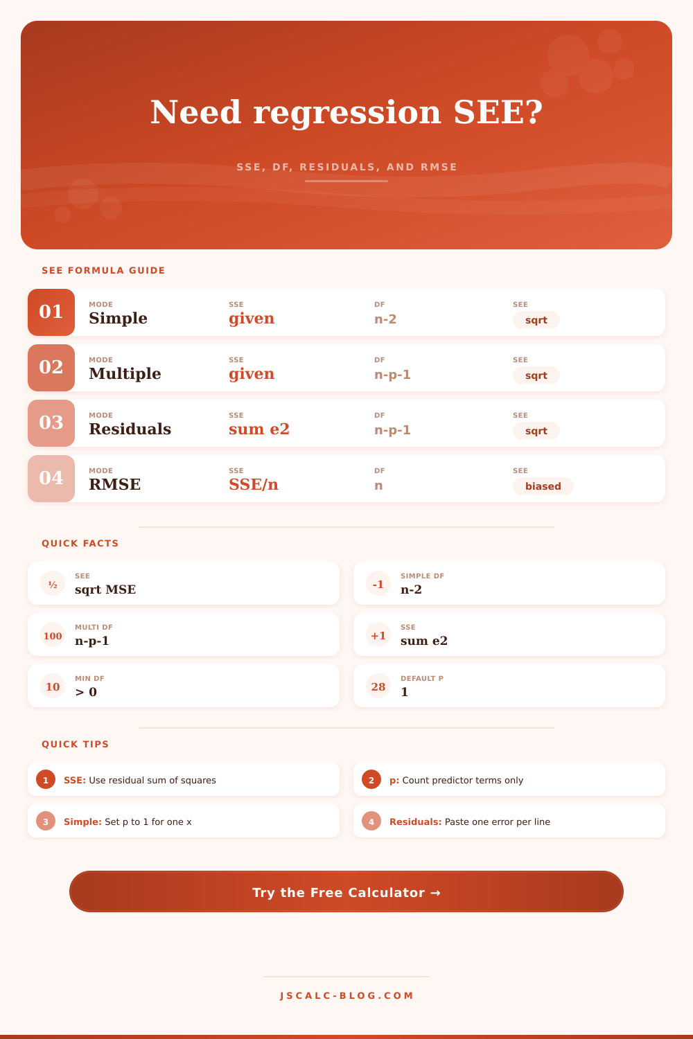
Simple regression uses df = n - 2.
SSE = sum of squared residuals. Disabled when residual list mode is selected.
For residual list mode, this is updated from the pasted residual count.
Count independent variables, not the intercept. Simple regression has p = 1.
Only used when regression type is set to entered residual df.
Shown beside SEE so reports keep the dependent variable unit.
Paste residual errors separated by commas, spaces, tabs, or line breaks. The calculator squares each value and sums them.
Estimate error results
| Method | Inputs needed | Degrees of freedom | Best used when | Watch for |
|---|---|---|---|---|
| Simple regression SEE | SSE and n | n - 2 | One x variable predicts y | Do not use n - 1 |
| Multiple regression SEE | SSE, n, and p | n - p - 1 | Several predictors are in the model | Count dummy columns as predictors |
| Residual-list SEE | Residual values and p | count - p - 1 | You have actual residuals instead of summary output | Keep residuals in response units |
| Direct residual df | SSE and residual df | Entered df | Software already reports error df | Match the same fitted model |
| RMSE | SSE and n | n denominator | Prediction-error summaries or ML reports | Not the unbiased regression SEE |
| Residual standard deviation | SSE and error df | same as SEE | Regression output labels sigma or RSE | Terminology varies by software |
| Model setup | n | p | Residual df | SEE denominator |
|---|---|---|---|---|
| Simple regression with one x | 24 | 1 | 22 | n - 2 |
| Two predictors plus intercept | 40 | 2 | 37 | n - p - 1 |
| Five predictors plus intercept | 96 | 5 | 90 | n - p - 1 |
| One numeric plus three dummy columns | 72 | 4 | 67 | n - p - 1 |
| Residual df reported by ANOVA table | not needed | not needed | given | entered df |
| Overfit or saturated model | 10 | 9 | 0 | not valid |
| Check | What it means | Good sign | Possible issue |
|---|---|---|---|
| Count | Number of pasted residuals | Matches the fitted sample | Missing or extra rows |
| Mean residual | Average signed residual | Near zero with intercept | Model omitted intercept or data mismatch |
| Largest absolute residual | Biggest miss in original units | Reasonable for the problem scale | Outlier or entry error |
| SSE | Sum of squared residuals | Matches regression output | Residuals pasted in standardized units |
| SEE | Typical vertical prediction error | Small relative to useful outcome scale | Model may be noisy for prediction |
| Output name | Formula | Unit | Plain-language use |
|---|---|---|---|
| SEE | sqrt(SSE / df) | y units | Typical fitted-value error after estimating parameters |
| SSE | sum e squared | y squared | Total unexplained squared error |
| MSE | SSE / df | y squared | Error variance estimate |
| RMSE | sqrt(SSE / n) | y units | Average prediction error with n denominator |
| Residual df | n - p - 1 | count | Observations left after fitting coefficients |
| Largest residual | max |e| | y units | Quick flag for unusual misses |
You might spend weeks checking your assumptions, fitting your models, and cleaning your data, only to have your actual predictions fall short (even with a perfectly straight-looking regression line). The disconnect between the two is often where concept of standard error of the estimate enters. Is it a measure of how well your model fits the data mathematicaly? No. Is it a measure of how confident you should be in trusting your predictions on new, unseen observations? Yes.
This is the beauty of the calculator. Plugging in either the raw residuals or sum of squared errors will do all the math for you. You won’t have to divide and square root things yourself, and it will make clear what this error mean for your particular dataset. It’s simpler than it sounds.
What is Standard Error of the Estimate?
The idea is this: how far off were you? On average. The SEE tell us about how far observations deviate from the regression line on average. For example, if you have an SEE of ten, then you should expect most of your predictions to fall in a certain range around true value, with your fitted line as center of that range.
That’s where things get tricky. What exactly does this mean? It doesn’t tell you anything about the intercept or the slope. It tells you something about the noise that was left behind once the model did its very best work. And that’s where folks mess up.
Most people makes a mistake in how they calculate degrees of freedom. To compute, you divide sum of squared errors by something called “degrees of freedom.” Not the sample size! For simple linear regression (one predictor), you take away two from your sample size, because you estimated a slope and an intercept. For multiple regression, you take away one more per each additional predictor.
If you don’t do that, then you’re using wrong denominator (the calculator figures that out for you automatically). That leads you to underestimate the error and overestimate your confidence: the model appears better than it actualy is. It is again just a little change, but it is important at modest sample sizes.
The tool takes your list of residuals, pastes it right into input box, then squares all of them and adds them together, applying degrees of freedom correction after that, which can come in handy if you’ve done regression analysis somewhere else and exported the residuals but forgot to export summary statistics. As long as you don’t paste in standardized residuals, just raw residuals, everything should work out fine.
The SEE has same units as your response variable. So if you’re predicting the price of houses in dollars, the SEE is also measured in dollars. Growth? Centimeters. It’s a very practical diagnostic because it’s so directly comparable. For example, if you’re predicting house prices in dollars, the SEE will be in dollars, making it easy to see how far off your predictions typically are.
For example, contrast this with root mean square error (RMSE), commonly used when discussing machine learning results. RMSE tends to be a little smaller then the SEE, and gets divided by the sample size. Also, RMSE can be biased downwards in small samples, while the SEE is an unbiased measure of the population error variance. You can observe how far apart they are on calculator.
The gap shrinks as you get into larger datasets, but in smaller studies, it reflects a true reduction in statistical rigor. The SEE is like a barometer for how reliable you think your model is. If the SEE compared to the range of your data is small, then the model is capturing the pattern in the data reasonably well. The larger the SEE, the more variation there is that isn’t explained by the predictors.
That doesn’t necessarily make the model worthless, just means that predictions will have wide confidence intervals. Report both this and your R-squared value, because sometimes you can have a high R-squared even with a large SEE when range of the response variable is really large.
In the end, then, your passion is tied to Earth by the standard error of the estimate. It’s a reminder that models are approximations; they’re not oracles. It quantifies how much wrongness you should of expected. It also guides your judgment about whether your model is accurate enough for the decision under consideration.
If you’re making predictions (e.g., sales) or if you’re evaluating a series of clinical trial results, understanding the margin of error matter as much as understanding the direction. The margin of error is what remains. As noise, once the model does its best.