Multiple Regression Coefficient Calculator
Enter a coefficient table row to compute the predicted Y change, t statistic, confidence interval, standardized beta, partial r, and two-tailed p-value.
Used for interpretation wording only; formulas stay the same.
Expected Y change for a one-unit increase in X, holding other predictors constant.
Use the coefficient standard error from the regression table.
Usually n minus all estimated model parameters.
CI is b ± t critical × SE_b.
The X change used for the unstandardized effect on predicted Y.
Needed for standardized beta; enter 0 if unavailable.
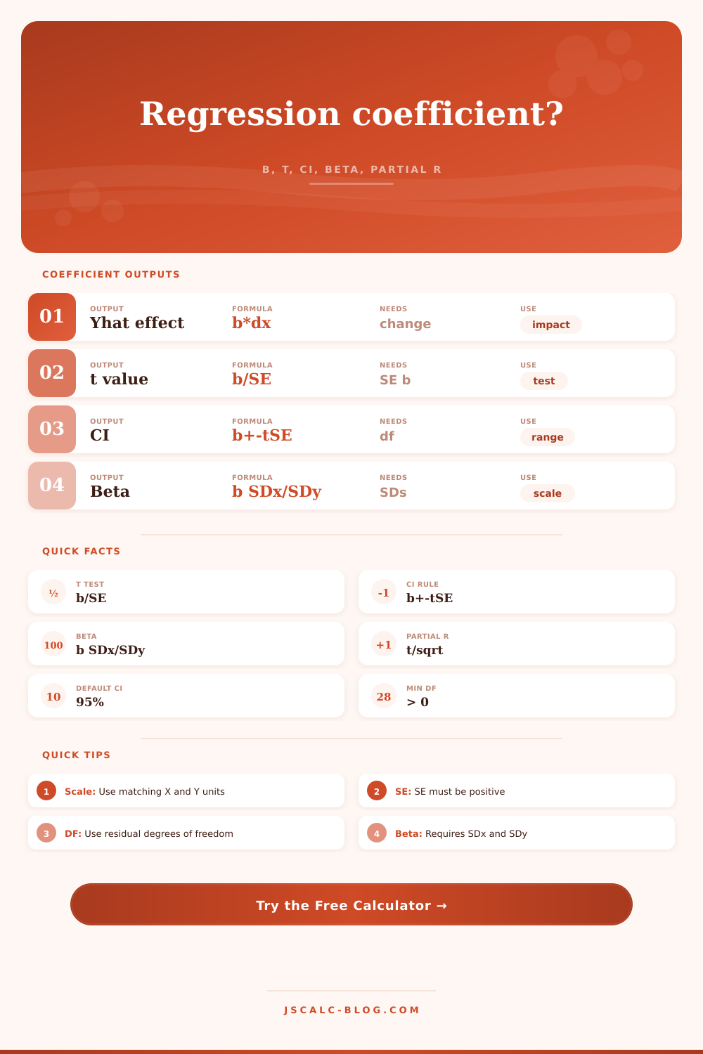
Standardized beta equals b × SDx / SDy.
Snapshot values update with the same coefficient row, so you can read practical impact, sampling uncertainty, and scale-free association together.
| Output | Formula | Required input | Interpretation | Regression note |
|---|---|---|---|---|
| Unstandardized effect | b × delta X | Coefficient and X change | Predicted Y change for the selected X movement | Holds other predictors constant |
| t statistic | t = b / SE_b | b and coefficient standard error | Distance from zero in standard error units | Uses residual df for inference |
| Confidence interval | b ± tcrit × SE_b | Confidence level, SE_b, df | Plausible coefficient range under the fitted model | Two-sided interval is standard |
| Standardized beta | b × SDx / SDy | Predictor and outcome standard deviations | Y standard deviation change per one SD of X | Useful for comparing predictors |
| Partial correlation | t / sqrt(t^2 + df) | t statistic and residual df | Unique association after other predictors | Sign matches the coefficient |
| Two-tailed p-value | 2 × tail area of t | t statistic and residual df | Evidence against b = 0 | Report with estimate and CI |
| Metric | Small cue | Moderate cue | Large cue | What to check |
|---|---|---|---|---|
| Absolute t | Below about 2 | About 2 to 3 | Above about 3 | Use df-specific critical value, not a fixed rule |
| Partial r | 0.10 to 0.29 | 0.30 to 0.49 | 0.50 or higher | Context and measurement reliability matter |
| Standardized beta | Below 0.20 | 0.20 to 0.49 | 0.50 or higher | Compare only within the same fitted model |
| CI width | Narrow vs scale | Touches zero | Very wide | Wide intervals usually mean low precision |
| Yhat effect | Small practical move | Useful shift | Decision-sized shift | Judge in outcome units, not just p-value |
| Sign direction | Negative slope | Near zero | Positive slope | Confirm coding and reference categories |
| Report piece | Example wording | Needs | Why it matters | Common omission |
|---|---|---|---|---|
| Coefficient b | Holding covariates constant, Y changes by b per X unit | Unit of X and Y | Preserves real-world scale | Leaving units unstated |
| Standard error | SE_b describes coefficient uncertainty | Model output table | Builds t and CI | Rounding too aggressively |
| Confidence interval | 95% CI for b = low to high | df and confidence level | Shows precision and compatible signs | Reporting p alone |
| Standardized beta | Beta compares predictors on SD scale | SDx and SDy | Scale-free within-model comparison | Mixing samples or transformations |
| Partial r | Partial r summarizes unique association | t and df | Converts coefficient test to effect size | Treating it as causation |
| Predicted change | A delta X change moves yhat by b times delta X | Meaningful X change | Translates slope into practical impact | Using one unit when it is tiny |
| Issue | Signal in calculator | Model check | Effect on coefficient | Next step |
|---|---|---|---|---|
| Multicollinearity | Large SE with meaningful b | VIF, tolerance, condition index | Inflates uncertainty and widens CI | Review correlated predictors |
| Suppression | Unexpected sign or beta | Zero-order vs partial associations | Coefficient may differ from simple trend | Inspect predictor relationships |
| Nonlinear effect | Yhat effect depends on range | Residual plots and added terms | Single b may average a curve | Try splines or transformations |
| Heteroskedasticity | SE source is unclear | Robust vs classical SE | t and CI change with SE method | Use the correct reported SE |
| Unit mismatch | Beta looks unrealistic | SDx and SDy units | Standardized beta becomes wrong | Use the same analysis sample |
| Small df | Large t critical value | Sample size and parameter count | CI expands quickly | Report df and avoid overclaiming |
On paper multiple regression is pretty cool. In practice, it’s more of a mess.
Here you get a bunch of numbers in a table: coefficients, standard errors, p-values. It feels like secrets of the universe are being revealed. But that table isn’t the territory, only a map. It reveal how variables move together. Not what that means for your actually decision. Your outcome could change by a fraction of a cent and yet still be statistically significant. The math care about it. Your wallet cares less.
What Multiple Regression Really Means
So what does it do? The calculator do the hard work after you input your regression results. After you enter raw values spit out by your regression software, it will convert those numbers to values you can apply in practice.
First, it needs you to input unstandardized coefficient (also known as b). This tells you how much your outcome is expected to shift when your predictor increase by one unit. One unit doesn’t sound too bad, but it’s worth noting that this could mean nothing to you in the real world. For example, if you’re trying to model salary as a function of years of education, then one year makes sense. However, if you’re attempting to model price of homes as a function of square footage, then a one-square-foot difference is an extremely small amount of space.
Therefore, the calculator prompt you for a value called delta X. Here, you can enter a more realistic increase, such as 500 square feet or ten years of experience. Then the calculator tell you what resulting impact on your predicted outcome will be.
The other key input is standard error, which indicates how far up and down that coefficient might bounce around if you repeated this study with another sample. A high standard error compared to the coefficient itself mean it’s a noisy result. Based off that, it creates what we call a confidence interval, a band of possible values for the true effect. If the interval contain zero, then you can’t say that the predictor reliably affects anything. It also calculates the t-statistic, the coefficient divided by its standard error. You can think of that as signal-to-noise ratio: The higher the t-value, the stronger the signal is versus the static.
Betas are standardized for comparison (with care). These eliminate units, which allows you to consider the relative size of various predictors alike. They require standard deviation values for the outcome and for each of the predictors. This tool will compute it for you, but the standard deviations should be from the same sample as the regression itself. Mixing samples is easy to do and will skew things.
Another good measure is partial correlation. This removes the impact of all other variables in the model, giving you the distinct association between one predictor and the outcome. This let you see what each variable adds on its own.
Here are the takeaways: these statistics are tricky to interpret. You’re probably thinking “significant” = “important.” But they aren’t the same thing. Even if you have a huge sample size, it’s possible to find small, unimportant differences and make them super-significant (i.e., the p-value < 0.05). It's also possible to have a big, real difference but fail to detect it due to low precision (wide confidence intervals). You want to focus on how much a change in the predictor affect the outcome. Is it something that moves the needle towards what you care about?
The real world doesn’t behave exactly according to a neat mathematical equation. Sometimes, you’ll run into multicollinearity. This mean your predictors are very strongly related to one another. This will increase the standard error of your coefficients and make them somewhat unreliable.
A bad model can’t be fixed by the calculator. It will only explain what your current model say. Are the signs counterintuitive? Are the confidence intervals large? That’s your cue to look more deeply at your data. Look for outlier points. Reread how you coded variables. Consider whether assumptions about linearity applies.
Regression isn’t a magic wand; it’s a way of understanding complexity. The bottom line is clarity. Will this change to an input probably create the outcome I want? How confident am I that this connection exists? Judgment fills the space between the math; the math establishes the limits.
Plug the figures into the machine; let it crunch the numbers; make the decision. It is a balance of logic and emotion. That’s where the true illumination occurs.