Logistic Regression Odds Calculator
Convert a fitted logistic model into log odds, odds, probability, odds ratios, and a 95% confidence interval for a chosen unit change.
Used only to label the breakdown.
Baseline log odds when predictors equal 0.
Also used for the odds ratio and CI cards.
Use the same scale used in the model fit.
Set to 0 if your model has one predictor.
Can be binary, centered, standardized, or raw.
OR = exp(beta1 x unit change).
For a 95% OR CI: exp(beta1 x d +/- 1.96 x SE x |d|).
Logistic model results
This table updates from the entered beta values and shows each term in the linear predictor before the logit is transformed.
| Term | Beta | Value | Contribution | Role |
|---|---|---|---|---|
| Intercept | -1.350 | 1 | -1.350 | Baseline |
| Predictor 1 | 0.420 | 2.000 | 0.840 | Focus OR |
| Predictor 2 | -0.280 | 1.000 | -0.280 | Adjustment |
| Total logit | sum | all terms | -0.790 | Predicted log odds |
| Logit | Odds exp(logit) | Probability | Odds wording | Use as a check |
|---|---|---|---|---|
| -3.00 | 0.050 | 4.7% | about 1 to 20 | rare event |
| -2.00 | 0.135 | 11.9% | about 1 to 7 | low event rate |
| -1.00 | 0.368 | 26.9% | about 1 to 3 | below even odds |
| 0.00 | 1.000 | 50.0% | 1 to 1 | null midpoint |
| 1.00 | 2.718 | 73.1% | about 3 to 1 | above even odds |
| 2.00 | 7.389 | 88.1% | about 7 to 1 | high event rate |
| 3.00 | 20.086 | 95.3% | about 20 to 1 | very likely event |
| Beta | OR exp(beta) | Odds change | Plain reading | Reverse beta |
|---|---|---|---|---|
| -1.386 | 0.25 | 75% lower | quarter the odds | 1.386 |
| -0.693 | 0.50 | 50% lower | half the odds | 0.693 |
| -0.223 | 0.80 | 20% lower | modest decrease | 0.223 |
| 0.000 | 1.00 | no change | null effect | 0.000 |
| 0.223 | 1.25 | 25% higher | modest increase | -0.223 |
| 0.693 | 2.00 | 100% higher | double the odds | -0.693 |
| 1.099 | 3.00 | 200% higher | triple the odds | -1.099 |
| 1.386 | 4.00 | 300% higher | quadruple odds | -1.386 |
| Confidence | Two-sided z | Log CI lower | Log CI upper | OR CI transform |
|---|---|---|---|---|
| 80% | 1.282 | b - 1.282 SE | b + 1.282 SE | exp(bounds) |
| 90% | 1.645 | b - 1.645 SE | b + 1.645 SE | exp(bounds) |
| 95% | 1.960 | b - 1.960 SE | b + 1.960 SE | exp(bounds) |
| 98% | 2.326 | b - 2.326 SE | b + 2.326 SE | exp(bounds) |
| 99% | 2.576 | b - 2.576 SE | b + 2.576 SE | exp(bounds) |
| Preset | Typical outcome | Predictor 1 scale | Predictor 2 scale | Reason to use |
|---|---|---|---|---|
| Credit Approval | approved | score bands | debt ratio | mixed signs |
| Subscription Churn | churned | complaints | tenure | risk rising |
| Clinical Screening | positive | marker units | age decades | clinical scale |
| Ad Click Model | clicked | relevance score | prior views | low base rate |
| Fraud Flag | flagged | risk score | account age | large OR |
| Admission Odds | admitted | GPA points | test score | interpretable OR |
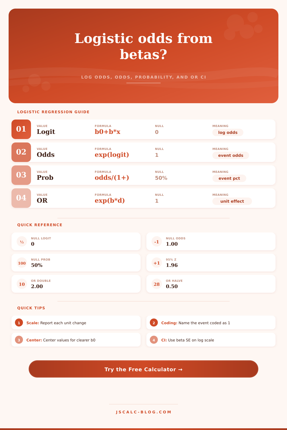
Core formulas used here: logit = beta0 + sum(beta*x), odds = exp(logit), probability = odds / (1 + odds), odds ratio = exp(beta*unit change), and OR CI = exp(beta*unit change +/- z*SE*abs(unit change)).
What’s behind all this? A logistic regression coefficient, while perhaps a confusing numerical value to you… Is fuel for prediction. It’s the unprocessed material that gets converted into a chance that something will happen or won’t.
The numbers you’re looking at when you examine model output are called log odds. They aren’t something your brain innately grasps. And because you think in terms of chances and probabilities, there’s a language barrier here. That’s where mistakes lie.
How to Turn Numbers into Chances
This calculator closes that divide, changing beta coefficients from any statistical program into the odds and probabilities you need to reach a decision.
Plug in your predictor coefficients and the intercept. You can think of the intercept as being the log odds when all your predictors is equal to zero. So this establishes starting point for calculating the rest. Then your remaining coefficients indicates the impact of each predictor on the odds for a one-unit increase in that variable.
In modeling credit approval, for example, your predictors may include income and debt ratio; in a clinical-screening application, they may include age and level of biomarkers. But what matters isn’t necessarily which variables you choose, it’s the scale! Knowing what a unit change represents in the real world helps you understand whether a coefficient of 5 is huge or small. A year-old patient? That’s nothing! A decade of life experience? Huge! The silent variable is always context, the thing that trips up most analyses. Define it.
Now that you’ve entered your numbers, the tool will transform them for you. Specifically, it will sum the linear predictor (the log of the odds) to obtain the logit. Then, it will take the exponential of this logit to obtain the odds. Lastly, it will convert these odds to a probability. This is helpful because it provides a step-by-step breakdown of how the math works out. This can help explain what’s going on.
For example, you might have a strong effect size, as shown by a high odds ratio, but baseline probability was already extremely low. This means the resulting actual risk may still be tiny. And that’s where folks mess up, conflating absolute risk with relative risk: A doubling of the odds, represented by an odds ratio of two, means you went from one in a hundred to two in a hundred. So yes, the risk is higher then it was, but in absolute terms, it’s still low.
But equally important: the tool also computes the confidence interval around the odds ratio. That’s what lets us interpret it correctly. Odds ratios are guesses (point estimates), but intervals are ranges of plausible values. Even if your point estimate is dramatically different from 1, if it falls within your interval, that means you found no evidence of an effect.
How does the calculator do that? It creates the interval on the log scale, then exponentiates those bounds. Why? Because you can’t just add/subtract the margin of error in odds ratio space. You need to let the math respect the fact that the odds ratio is based off logs. The tool does this for you.
The page has some sanity checks in the form of reference tables that you should take a peek at. They will tell you: when your logit is -3, it’s below a five percent probability; when your odds ratio is 0.5, you’re talking about half the odds. They’ll let you know when your number was entered correctly. They will also catch data entry mistakes while they are still manageable, rather than after they have spread through a whole report. It is a little thing, but it’s worth it, since finding one misplaced decimal point or a flipped sign can save hours of reworking.
But where it gets powerful is when you play with the unit change. You don’t have to assume one dollar changes; you can say, I’d like my predictor to be income, and I’d like the odds ratio to reflect what happens if income goes up by ten thousand dollars rather than just one. The tool will let you do that, it will recalculate the odds ratio and its confidence interval at whatever new scale you’ve chosen. That way, the results make sense in terms of what matters to your audience.
A stakeholder wants to know how something impacts their life, which means they care about a meaningful change to a policy, not a marginal unit of change.
The key here is to shift perspectives on what you’re seeing… It’s no longer about those coefficients, now you have the probability of an event occurring based on certain conditions. Probability is the answer so the probability output provides exactly that. Odds ratios and log odds are the path but probability is the destination and therefore the final answer.
Run through various scenarios, adjust the predictor values and observe the impact on the probability output. Observe how sensitive your model is and whether its outputs is driven by one or two variable or multiple. That analysis, the sensitivity analysis, is as informative as, if not more than. The fit itself. The scale of the variables matters more then the specific variables themselves. The numbers won’t lie but you can be led astray if you fail to ask the appropriate questions. Begin with the probability and finish with the decision; that’s where you take statistical information and convert it to strategy.
You should of used this tool earlier! Actualy, finding one misplaced decimal point or a luxuriously complex error could save hours of reworking.