Regression Prediction Calculator
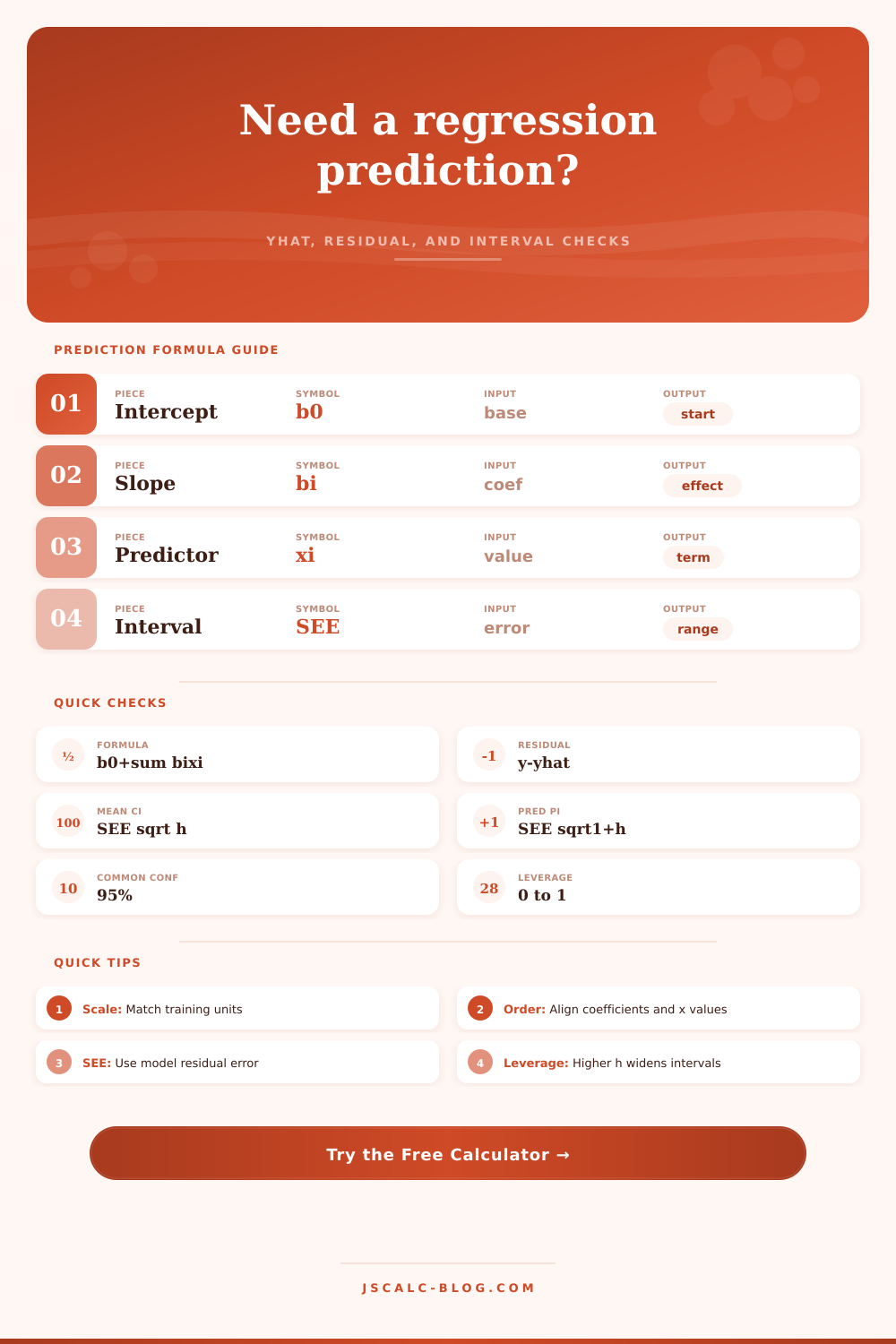
Compute yhat from an intercept, matched coefficient and predictor lists, observed residuals, and optional SEE plus leverage interval components.
Used for interpretation text only; the formula stays the same.
Baseline prediction when every predictor equals zero.
Separate values with commas or spaces. Order must match the predictor list below.
Use the same units and coding scheme used when the regression model was fit.
Leave blank if you only need the forecast.
This powers the optional mean CI and prediction interval.
Typical in-sample h is near p / n; higher leverage widens intervals.
Uses a normal critical value approximation for browser speed.
| Term | Coefficient bi | Predictor xi | Product bi x xi | Share of yhat |
|---|---|---|---|---|
| x1 | 3.2 | 10 | 32 | sample |
| Input | Symbol | Used In | Typical Source | Quality Check |
|---|---|---|---|---|
| Intercept | b0 | Point prediction | Model output table | Keep original scale |
| Coefficient list | b1...bk | Term products | Regression coefficients | Match x order exactly |
| Predictor list | x1...xk | Term products | New observation row | Use training units |
| Observed outcome | y | Residual check | Actual measured result | Leave blank for forecast |
| Residual error | SEE | Intervals | Model summary output | Must be nonnegative |
| Leverage | h | Intervals | Hat matrix diagonal | Higher h means wider range |
| Interval Type | Standard Error | Formula | Narrow When | Interpretation |
|---|---|---|---|---|
| Mean response CI | SEE x sqrt(h) | yhat +/- t x SEmean | h is small | Uncertainty in average y at this x |
| New prediction PI | SEE x sqrt(1 + h) | yhat +/- t x SEpred | SEE is small | Range for one new observation |
| Residual screen | SEE | residual / SEE | near zero | Standardized miss check |
| Leverage screen | h | about p / n baseline | near baseline | Flags unusual predictor rows |
| Critical multiplier | z approx | 80% to 99% | lower confidence | Controls range width |
| Preset | Predictors | Intercept | Coefficient Pattern | Best Use |
|---|---|---|---|---|
| Retail sales forecast | Traffic, ads, price, promo | 120 | mix positive and negative | Short-term demand checks |
| Home value model | Area, beds, age, school | 55 | large area effect | Appraisal sanity check |
| Exam score prediction | Study, attendance, prior, sleep | 18 | all positive | Education planning |
| Manufacturing yield | Temp, speed, pressure, defect | 88 | defect negative | Process monitoring |
| Energy demand | Temp, occupancy, weekday, area | 35 | thermal load heavy | Facility load estimates |
| Customer churn risk | Tickets, tenure, use, plan | 12 | risk score scale | Retention triage |
| Crop yield estimate | Rain, nitrogen, heat, density | 22 | stress negative | Field comparison |
| Delivery time model | Distance, stops, traffic, crew | 8 | crew negative | Route planning |
| Lab calibration line | Signal, blank, drift | 0.4 | signal dominant | Instrument conversion |
| Diagnostic | Low Range | Moderate Range | High Range | Action |
|---|---|---|---|---|
| Absolute residual / SEE | 0 to 1 | 1 to 2 | above 2 | Check unusual miss |
| Leverage h | 0 to 0.05 | 0.05 to 0.20 | above 0.20 | Confirm x is in-domain |
| Prediction SE / SEE | near 1.00 | 1.02 to 1.10 | above 1.10 | Expect wider interval |
| Largest term share | under 40% | 40% to 70% | above 70% | Inspect dominant driver |
| Coefficient sign mix | stable | mixed | unexpected | Review coding direction |
There’s the coefficients. There’s the intercept. There’s that new data point staring back at you from the screen. And the math? It’s pretty easy, almost too easy. Multiply each coefficient by its corresponding predictor value, then sum the products. Add the intercept. Boom. There’s your yhat, your predicted result.
In fact, it’s deceptively simple arithmetic, which is precisely where the trap lies. The actual prediction work of regression has nothing to do with the math itself. It has nothing to do with the calculation. It is everything to do with judgment call around it. You must recognize that a number that appears correct on the spreadsheet could be flat-out wrong out in the real world.
Why the Math Is Not the Hardest Part
Yet most people think the point estimate, the single number; is the entire story. That’s why they want it. It seems definitive. Without some notion of uncertainty, though, a prediction is just a guess with more steps involved. And although the calculator will multiply for you, you should of know what those numbers mean in reality.
What does the intercept represent? It represents the baseline: the predicted value if all predictors equals zero. This situation is impossible for most models. This might be a student who studied for zero hours or a house that has zero square feet. You don’t have to be able to make physical sense of the intercept. You simply need it to serve as an anchor, so that slopes can do their jobs.
That’s where the intuition comes from: the coefficients. They tells you how many more (or fewer) units are sold when that particular predictor shifts by 1 unit. But this only works if you hold everything else constant. That’s a fragile all-else-being-equal assumption. It means you’re assuming a static world except for that single variable you’re trying to tweak.
For example, in retail, you can buy an ad that drives sales… but only if there’s some inventory left. If you sell out of stock, then your coefficient for ads isn’t worth squat. The model doesn’t know you’ve sold out of stock. It just spits out the number based on what it knows about how things were related in the past. You need to bring in missing context that the model doesn’t have.
And order does matter, different than what many people believe. The coefficients and the predictor values needs to be exactly lined up when you enter them into a list and feed them to a calculator. The first coefficient needs to match with the first predictor value. If you accidently switch the two around, the math will run without complaint. But it’ll give you nonsense. The calculator won’t complain about whether or not your input makes any sense. Only that the syntax matches. And that’s why human oversight is non-negotiable.
You must trace each coefficient back to the source variable. Did you train the model using temperature in degrees Celsius but then used degrees Fahrenheit for your test data? Did you put in raw counts rather than percentages? Those scale mismatch things kills an accurate prediction, and silently so.
And what about range? When you build a model, you have to realize that it’s only good inside of range of the data used to construct it. When you go beyond the range, you’re doing an extrapolation, which is generally a poor idea. What happens is that the relationship between variables may be linear at the core, but curves off as you move out to the extremes. You may have a sales model where ad budgets work fine when they’re modest, but when you get to a million bucks, you see diminishing returns set in pretty hard. Linear equations doesn’t bend to match this reality. They simply continue upward.
The leverage statistic is helpful in identifying these extreme points. If you’ve got high leverage, you’re way out on the fringe relative to your data. Be warned. Your prediction isn’t grounded.
That’s not a bug. That’s a feature. Reality isn’t certain. What are the two things the prediction interval covers? One: The uncertainty in the estimated coefficient(s). We don’t know what the actual slope of the universe is. We have an estimate. Two: the natural scatter of individual observations. Even assuming we were able to estimate the true line precisely, individuals still bounce around it. The prediction interval is broader then the confidence interval for the mean because it needs to account for the individual bouncing around. You get a false sense of precision if you ignore that.
Use the tool to do the work for you. Let it compute the intervals. Let it sum up the terms. But maintain your focus on the logic. Verify the ranges. Verify the units. Does this make sense as a group of predictors? Is the number just the beginning of a discussion or its end? Use a simple sum at the beginning and a decision at the end. Ensure that the decision is not based off anything other than arithmetic.