Covariance Calculator
Calculate sample covariance, population covariance, Pearson correlation, and the least-squares regression line from paired x and y observations.
📌Covariance Presets
🧮Paired Data Inputs
Use sample for observed data drawn from a larger process; use population for a complete finite set.
This is the predictor axis for the regression slope.
This is the response axis used for the fitted line.
Paste values separated by commas, spaces, tabs, or line breaks.
The first y value pairs with the first x value, and so on.
📋Summary Grid
🔍Paired Data Breakdown
Contribution table
Summary statistics table
Regression diagnostics table
📐Formula Reference
| Quantity | Formula | Denominator | Meaning | Report when |
|---|---|---|---|---|
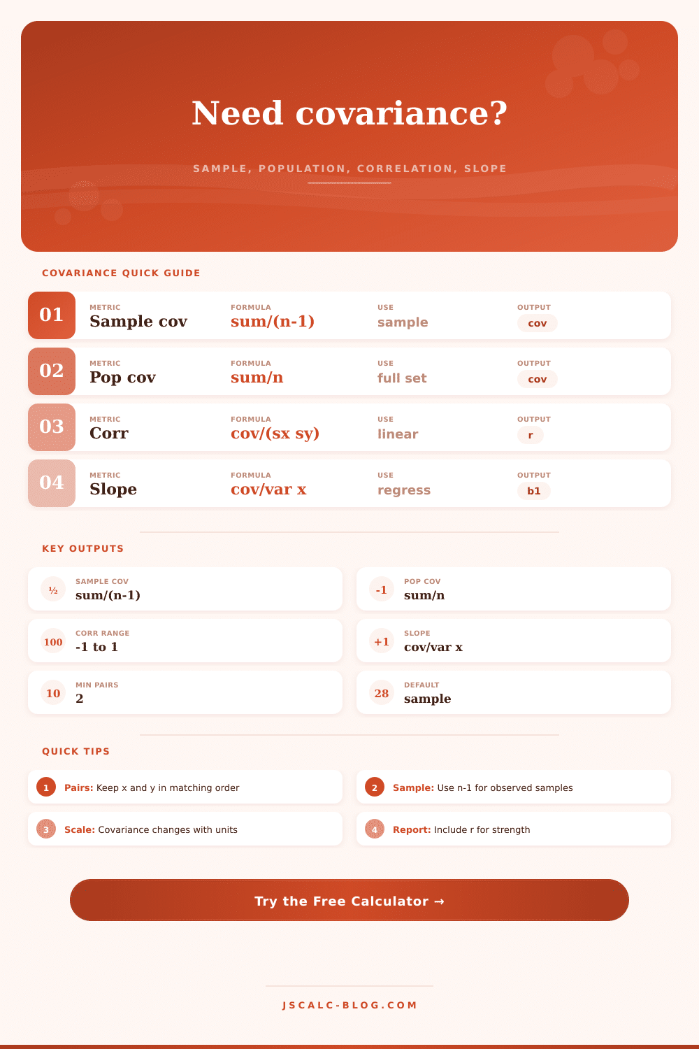
| Sample covariance | sum((x - xbar)(y - ybar)) / (n - 1) | n - 1 | Joint movement in original units | Data are a sample |
| Population covariance | sum((x - xbar)(y - ybar)) / n | n | Complete-set joint movement | Data are the full population |
| Correlation | cov / (sx x sy) | matching method | Unitless linear association | Compare strength across variables |
| Regression slope | cov / var x | matching method | Change in y for one x unit | Predict y from x linearly |
| Intercept | ybar - slope x xbar | none | Fitted y when x equals zero | The zero point is meaningful |
| R squared | r x r | none | Linear variation share | Describe simple linear fit |
📚Interpretation Tables
| Result pattern | Covariance sign | Correlation sign | Regression slope | Plain interpretation |
|---|---|---|---|---|
| Move together | Positive | Positive | Positive | Higher x tends to pair with higher y. |
| Move opposite | Negative | Negative | Negative | Higher x tends to pair with lower y. |
| Flat linear signal | Near zero | Near zero | Near zero | The linear pairing is weak in this data. |
| Scale-sensitive | Large units | Unchanged | Changes by units | Covariance depends on measurement scale. |
| Perfect line | Nonzero | Exactly 1 or -1 | Exact linear slope | All points fall on one straight line. |
| No x spread | Undefined slope | Undefined | Undefined | x variance must be greater than zero. |
Covariance is a measure of how two variable change together. It tells you that they’re related, but it doesn’t eliminate the units of measurement. If one is revenue (in thousands) and another is ad spend (in dollars), then the resulting value will be a mix of unit. That’s fine for predicting values, but clumsy for comparing them to other things like crop yield versus rainfall.
For comparison purposes, we need different metric. That’s where correlation comes in. It removes units and gives you a pure measure of linear strength. Its value is always between -1 and 1. In other words, correlation is cleaner measure for comparison; covariance are the workhorse for prediction.
How to Use the Covariance Calculator
After entering two set of observations, the calculator do the math. Simply enter your y values and your x values in same order. It doesn’t matter if your x is on top or bottom, it just needs to be the same order as your y. Get that wrong and you’re matching the relationship of totally different pairs of events.
By default, the calculator take your data to be a sample from some larger set. That’s why the formula use n-1 in the denominator, adjusting for the bias of any small sample. In case you have all population data, say for every employee at a small business, then you toggle to population option. That switches the denominator from n-1 to n, changing result.
This regression slope tends to be most useful result. It represents the amount we expect y to shift for every one unit increase in x. It’s just the covariance of x and y, divided by variance of x. In this ratio, the numerator and denominator cancel out. The same slope results whether you use population or sample versions of each term. That means that no matter what you choose for the denominator, the slope will be robust.
The intercept simply anchors the line as it predicts what value of y would correspond to an x-value of 0. If you think it’s reasonable for x to ever equal zero in your context then go ahead and use the intercept. For example, maybe you want to predict revenue with zero ad spend, that might make sense. But predicting a person’s height at zero years old? Not so much.
These results is highly sensitive to outliers. Because covariance uses the product of deviations, one extreme observation can tug everything in its direction. A week where revenue was lower than expected despite a big ad spend will result in a large negative product of the deviations. Even though the other weeks might exhibit a clear trend, that single point can undermine what seems like a strong correlation.
In the results section, there is also a table that breaks down how much each pair contribute. By looking through that table, you should be able to identify which observations is pushing the relationship. If one week accounts for most of the sum, then you know something to be wary of when interpreting result.
A lot of folks will see the covariance number and attempt to read right off it what it means. “Covariance of 50! That’s bigger than covariance of 5.” Uh oh. Your intuition is wrong if your variables are on wildly different scales. Correlation corrects for this. The variables could be anything, like dollars and years. Grams and centimeters? A correlation of 0.8 means a strong positive relationship.
R squared just equals the correlation times itself. What does R squared tell you? It tells you how much of the variance in y is explained by x. If R squared = 0.64, then 64% of the variation in y can be associated linear with x. The remainder is not captured (noise) or captured but not linear (non-linear effects).
The first thing to check on a scatter plot when making a model: do the points drift up? Down? Flat? Upward drift mean positive covariance and a positive slope. Downward means negative for each. A cloud of points in any direction at all means close to zero. You can get these answers immediately from the calculator, but your task is to make sure input matches up. Are the pairs lined up correctly? Are your data a whole or a sample? Do you have outliers which skew the mean? Tick the boxes and then watch as the math shows the hidden structure.
You aren’t simply crunching numbers, you’re tracing the invisible thread tying two variables together. Not only do you get a coefficient, but you understand the strength, the reality and whether it’s useful for whatever decision should of happen next.