Partial Correlation Calculator
Estimate the correlation between X and Y after adjusting for one or more control variables, then test it with t, df, p-value, confidence interval, and effect-size context.
Correlation between X and Y before adjusting for Z.
Correlation between X and the control variable or score.
Correlation between Y and the control variable or score.
Use the complete-case sample used for all correlations.
Direct df supports multiple controls from regression output.
For one Z variable, k = 1 and df = n - k - 2.
Used for the decision rule and confidence interval.
Most reports use the two-tailed option unless the direction was planned.
Calculations use full precision; this only changes display rounding.
| Absolute partial r | Common label | Partial r squared | What to inspect next |
|---|---|---|---|
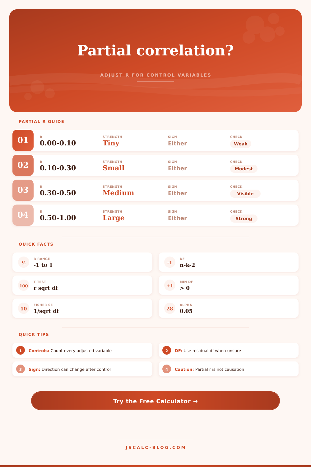
| 0.00 to 0.10 | Tiny | 0% to 1% | Check whether the control removed nearly all association. |
| 0.10 to 0.30 | Small | 1% to 9% | Look at confidence interval width and design power. |
| 0.30 to 0.50 | Moderate | 9% to 25% | Report both the adjusted and zero-order correlations. |
| 0.50 to 0.70 | Large | 25% to 49% | Check scatterplots and nonlinear patterns carefully. |
| 0.70 to 1.00 | Very large | 49% to 100% | Screen for duplicated measures or near-collinearity. |
| DF situation | How to enter it | Why it matters | Example |
|---|---|---|---|
| One control variable | Mode: controls, k = 1 | Matches the standard three-correlation formula. | Height adjusted for age |
| Several controls | Mode: controls, k = number adjusted | Uses df = n - k - 2 for the t test. | Age, income, baseline score |
| Regression output | Mode: direct residual df | Supports models where df is already known. | Software reports df = 84 |
| Small sample | Use exact n and k | Small df makes p-values and intervals wider. | n = 18, k = 3 |
| Missing data | Use complete-case n | Pairwise correlation counts can overstate df. | n differs by variable pair |
| Diagnostic check | Healthy pattern | Warning pattern | Action |
|---|---|---|---|
| Control relevance | Z relates to X or Y | Z unrelated to both | Question whether the control belongs in the model. |
| Collinearity | |r_xz| and |r_yz| below about 0.80 | Near 1.00 with either variable | Inspect variance inflation or measurement overlap. |
| Sign reversal | Adjusted sign is expected | Partial r flips direction | Look for suppression, confounding, or coding errors. |
| Linearity | Residual plots roughly linear | Curved residual pattern | Consider transforms or rank-based alternatives. |
| Outliers | No single point drives the result | One case changes r greatly | Run influence checks and robust sensitivity analyses. |
| Use case | X and Y | Controls | Report wording | Common caveat |
|---|---|---|---|---|
| Education | Study and score | Prior GPA | Adjusted association remains | Motivation may still confound |
| Health | Exercise and BP | Age, BMI | Association after controls | Medication history matters |
| Marketing | Spend and sales | Season, traffic | Net linear relationship | Campaign timing may lag |
| Finance | Income and saving | Age, dependents | Controlled correlation | Outliers can dominate |
| Biostatistics | Dose and response | Baseline level | Adjusted dose-response link | Nonlinearity may be hidden |
| Operations | Training and output | Tenure, team | Partial r with df | Nested teams need care |
If you believe there is some sort of third-party factor that explains relationship between two variables (e.g., you think discipline, not study time, drives exam performance), then partial correlation allow you to hold that variable constant in order to assess whether the relationship remains significant. In other words, it strips out common variation with your control variable and displays the unique linear connection between X and Y.
As long as you know sample size and the zero-order correlations, the calculator (above) do this math for you. No need to derive formula yourself. It’s based on three Pearson correlation coefficients: one that links X and Y; another that links X and the control variable Z; and yet a third that links Y and Z.
What Is Partial Correlation?
If latter two are both strongly associated with Z, the partial correlation should decreases from its initial amount. And that decrease is what calculation aims to demonstrate. Is there additional information in X that contributes to an understanding of Y over and beyond that which can be gathered from Z?
Remember, garbage in, garbage out. How does it affect what you input? Since you are calculating three correlation coefficients from the same group of cases, you want those cases to be represented as accuratey as possible in each calculation. That’s why missing data can be a problem. It could result in pairwise calculations using different subsets of your data and thus inflate number of apparent degrees of freedom.
Because of this, tool also has a mode for entering degrees of freedom directly. If you’ve run your regression outside of the tool and have an estimate of the residual df value, you can avoid having the tool calculate it. This is useful when dealing with complex models where raw count does not necessarily represent effective sample size.
The conclusion isn’t just “p-value below.05 so we did something.” Is.3 (i.e., partial correlation of 0.30) small? Yes, that’s small. It also show that even after controlling for the confounder, the two variables still share nine percent of their variance. That’s a sizable chunk of explanatory power, particularly in context of health metrics or social science.
That number can be turned into intuition using reference tables on the interface. Those tables will tell you what counts as big, what counts as little, what’s artifact and what’s substance. But that doesn’t mean that big = true. You should of still examine whether the control variable has suppressed the relationship by obscuring its actualy nature.
When the sign changes on the partial correlation, then the confounder likely had an opposing effect. Like regular Pearson correlation, partial correlation rely on two assumptions: equal variance and linearity. If relationship between variables is curved different than linear, then the adjusted coefficient could be misleading. Also, outliers will impact the variance and skew outcome.
The tool includes confidence intervals so you can judge how precise estimate is. That’s important with small samples when the t-statistic bounces all over the place. If the interval is wide, it means your result require replication. On its own, it’s too noisy to represent a definitive answer.
Statistics are sometimes viewed as a gatekeeper with binary output: Yes or No. Think of partial correlation more like a lens, it illuminates. It does not imply causation. It doesn’t remove the need for careful experimental design. Instead, it provides an answer to this question: “Is there relationship between these two variables controlling for this particular variable?”
In some cases, that relationship dissapears completely. That’s validation that you were correct in suspecting that the confounder was responsible. In other instances, the relationship hold up strongly. That indicates you can have confidence that the association between X and Y is valid.
In either case, you’ve gone from guessing to knowing. The equation itself isn’t complicated; deciding which control variable matters most are the hard part.