Redshift Calculator
Calculate redshift from rest and observed wavelength, solve the missing wavelength, compare low-z and relativistic recession velocity, and read scale factor, stretch, distance, and uncertainty.
| Spectral Feature | Rest Wavelength | Common Use | Line ID Caution |
|---|---|---|---|
| Lyman-alpha | 121.567 nm | high-z galaxies and quasars | absorbed by neutral hydrogen forests |
| O II doublet | 372.7 nm | star-forming galaxies | can blend at low spectral resolution |
| H-beta | 486.133 nm | Balmer emission and absorption | near O III in many spectra |
| O III | 500.684 nm | nebular emission and AGN | often paired with 495.9 nm line |
| H-alpha | 656.281 nm | nearby galaxy redshifts | watch N II contamination nearby |
| HI 21 cm | 21.106 cm | radio galaxy gas redshift | velocity convention may differ |
| CO J=1-0 | 2.60076 mm | molecular gas in galaxies | higher-J lines can be confused |
| CMB peak proxy | 1.063 mm | thermal background stretch | use as a scale example only |
| Redshift | 1 + z | Scale Factor | Wavelength Shift |
|---|---|---|---|
| -0.01 | 0.99 | 1.0101 | 1 percent blueshift |
| 0.01 | 1.01 | 0.9901 | 1 percent redshift |
| 0.10 | 1.10 | 0.9091 | 10 percent longer wavelength |
| 0.50 | 1.50 | 0.6667 | visible lines move infrared |
| 1.00 | 2.00 | 0.5000 | wavelength doubles |
| 3.00 | 4.00 | 0.2500 | Lyman-alpha to visible band |
| 6.00 | 7.00 | 0.1429 | reionization-era galaxy scale |
| 1100 | 1101 | 0.0009 | CMB-era stretch example |
| z | Approx v = zc | Relativistic beta | Difference |
|---|---|---|---|
| 0.001 | 300 km/s | 0.0010 c | negligible |
| 0.010 | 2,998 km/s | 0.0100 c | tiny |
| 0.050 | 14,990 km/s | 0.0488 c | about 2.4 percent |
| 0.100 | 29,979 km/s | 0.0950 c | about 5 percent |
| 0.500 | 149,896 km/s | 0.3846 c | approx overstates |
| 1.000 | 299,792 km/s | 0.6000 c | approx breaks down |
| Observation Band | Typical Range | Redshift Use | Example |
|---|---|---|---|
| Optical | 350-900 nm | nearby emission lines | H-alpha at z below 0.37 |
| Near infrared | 0.9-2.5 um | z near 1 to 6 line work | Lyman-alpha at z about 6 |
| Mid infrared | 2.5-25 um | dusty or high-z features | H-alpha at z above 3 |
| Millimeter | 0.3-10 mm | molecular lines and CMB | CO ladders in galaxies |
| Radio | cm to m | HI 21 cm redshifts | neutral gas surveys |
That’s where Redshift comes in. It is sort of like Doppler shift, except instead of moving closer or farther from an object, we’re stretching out wavelength of light as space itself stretch over the course of billions of light years. And what you see when you look at a galaxy isn’t a snapshot so much as a timestamp, a timestamp that calculator can turn back into distance, scale factor, and velocity.
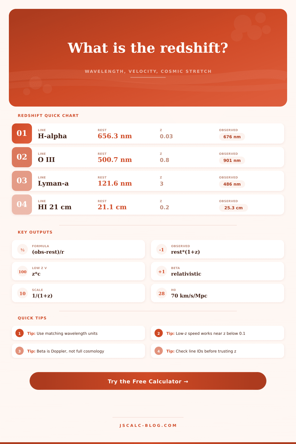
But first you need to know what those numbers mean; what the universe do to the light before it hits your sensor. What’s the starting point? That would be the rest wavelength, the lab standard for a given spectral line (e.g., Lyman-alpha or H-alpha). That’s the wavelength of element in its pure form. What you observe is different: that’s the wavelength. The gap between those two wavelengths are called redshift (z).
What Is Redshift?
So if measured wavelength is twice as long than the rest wavelength, then z = 1. That means the universe have expanded by a factor of two since light was sent out. You pick proper rest wavelength and the calculation does the work.
One mistake amateurs often make in spectroscopy is to misidentify the line. Hydrogen may look like oxygen. Oxygen can masquerades as hydrogen. Check accompanying lines to confirm.
For nearby galaxies, the low-redshift (near zero point one) version approximate recession velocity by multiplying z by speed of light. So you can just multiply z by the speed of light and get an approximate result. That won’t work at high values of z. Here’s why: space is expanding enough that simple linear mathematics are no longer right. At higher values, it use relativistic beta calculations to give a better sense. Applying the low-z version to a faraway quasar would greatly exaggerate its rate of travel. The calculator split them up so you can visualize the impact. It shows where common-sense ideas of motion break down in universe-wide setting.
One other key result is scale factor, which is proportional to size of the universe back then compared to now. If redshift is a value of 3, the universe had shrunk down to a quarter of its present size. So that puts some concrete meaning on those abstractions. It’s about history of expansion rather than just the rate.
These reference tables shows the shifting of various spectral lines with increasing redshift and band. For example, H-alpha shift to infrared at modest redshifts. That explains why you need near-infrared cameras to study early universe. The light is still there, but it shifted outside visible range.
These are all very uncertain measurements. At high z, an error of a few nanometers become a big error in the redshift value. Line identification can be unclear due to poor spectral resolution. You can enter the wavelength measurement uncertainty into calculator and see if it affect your result. If the error bars intersect with other potential line identifications, then your exact redshift value is misleading. Accuracy isn’t the same thing as precision. This is important for those dealing with spectal data. It forces you to admit the limitations of your measurement.
Lastly, we have an approximate measure of distance from the Hubble distance estimate. This use the Hubble constant to provide a kind of yardstick, though this view is simplified because it does not account for how matter and dark energy are spread across space. It provides a basis for the idea that redshift is about space rather than just time: you are observing an object located at that distance.
But how do wavelength, velocity and scale factor relates? How does the universe expand? The answers let you go from raw numbers to meaning behind them. And that’s what redshift represents. A look back in time, except that the universe has expanded since then, so it has stretched the wavelengths.