Transit Depth Calculator
Estimate exoplanet transit depth from planet and star radius, then convert the signal into percent, ppm, mmag, blended depth, grazing depth, and observing signal-to-noise.
Transit depth = (Rp / Rs)2 × 100%
Rp and Rs must be in the same radius unit. The calculator converts both radii to kilometers, squares the radius ratio, converts the result to percent and ppm, then applies optional grazing and blend dilution adjustments. The mmag output uses −2.5 log10(1 − depth) × 1000.
| Scenario | Planet Radius | Star Radius | Depth | PPM |
|---|---|---|---|---|
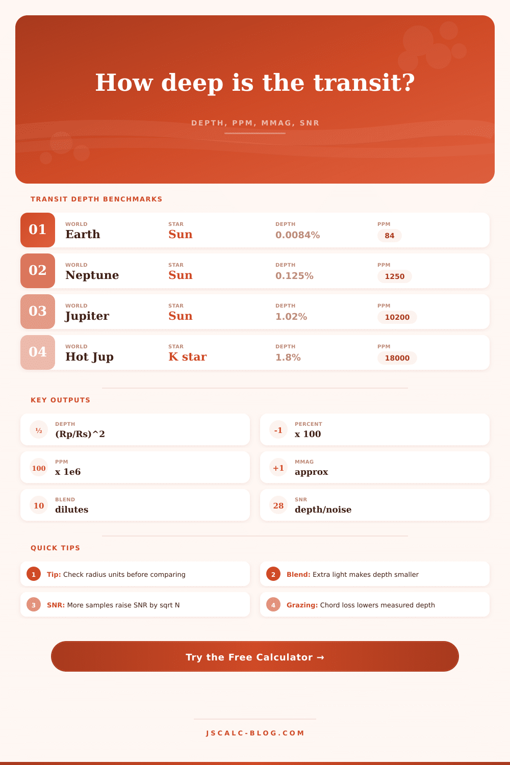
| Earth-size planet around Sun-like star | 1.00 R⊕ | 1.00 R☉ | 0.0084% | 84 ppm |
| Super-Earth around small M dwarf | 1.50 R⊕ | 0.20 R☉ | 0.472% | 4,720 ppm |
| Neptune-size planet around Sun-like star | 3.88 R⊕ | 1.00 R☉ | 0.126% | 1,260 ppm |
| Jupiter-size planet around Sun-like star | 1.00 Rj | 1.00 R☉ | 1.008% | 10,080 ppm |
| Inflated hot Jupiter around K dwarf | 1.35 Rj | 0.75 R☉ | 3.27% | 32,700 ppm |
| Small planet around TRAPPIST-1-like star | 0.92 R⊕ | 0.12 R☉ | 0.494% | 4,940 ppm |
| Observed Depth | Per-Point Noise | Samples | Estimated SNR | Reading |
|---|---|---|---|---|
| 80 ppm | 50 ppm | 100 | 16.0 | Space-quality Earth analog signal |
| 500 ppm | 300 ppm | 80 | 14.9 | Strong small-planet detection |
| 1,200 ppm | 800 ppm | 70 | 12.5 | Typical Neptune-class signal |
| 10,000 ppm | 2,000 ppm | 40 | 31.6 | Deep hot-Jupiter event |
| 300 ppm | 1,000 ppm | 60 | 2.3 | Likely needs more data |
| Adjustment | Calculator Factor | What It Represents | Depth Effect |
|---|---|---|---|
| Central transit | 1.00 | Planet crosses a bright central chord | Full geometric depth |
| High impact | 0.82 to 0.93 | Shorter chord and stronger limb-darkening sensitivity | Moderately reduced depth |
| Grazing chord | 0.58 to 0.74 | Only part of the planet disk covers the star | Depth can be much shallower |
| Blend dilution | 1 / (1 + blend) | Nearby star adds flux inside the aperture | Observed dip is reduced |
| Combined effect | grazing × dilution | Both geometry and extra light are present | Use observed depth for SNR |
The light from an exoplanet transit is quite faint. When animations depict transits, they makes it seem like planet blocks out the star like a dark circle. That’s not exactly what happens.
What you’re trying to detect is a decrease in brightness that might only amount to one part in ten thousand or so. These aren’t clean-cut blockages (which makes them easy to visualize), this is a search for tiny signal against a noisy background.
How to Measure Light from Planets
Before going to observe, you need to calculate roughly how deep that transit should of be. The calculator will do the geometry for you. Plug in your radii and get back your signal-to-noise ratio and other thing (in parts per million).
It’s also pretty easy to do the math. The transit depth (the fraction of the star covered) is proportional to the ratio of the areas of the planet and star. And area is proportional to square of the radius. So even a tiny difference in radius makes a big difference in the signal. For example, if a planet were twice as large as it was, the depth would go up by a factor of four. If it were 4 times bigger, the depth would be 16 times deeper.
That’s why people gets confused about how hard it should be to detect something based off its radius. The tool normalizes the planet and star radius to same unit. It then takes the square of that ratio to give you desired depth.
The desired depth isn’t always what you see. However, telescopes must also contends with noise. The other input addresses the noise. How good is your detector? Photometric noise per exposure limit detection ability. Even a good transit may be deep, but an unstable light curve will lose the signal.
Set the number of exposures (and change the noise value) while transiting. Remember, signal-to-noise grow as the square root of the sample count. Getting double the integration time only gives ~forty percent better signal-to-noise. Poor precision requires lots of data. Ground-based observers face a tough tradeoff.
Things get more complicated when you blend and graze events. When another star is in the field of view, its light dilute the transit signal. A ten percent blend will reduce the measured depth about ten percent. Small planet candidates is especially sensitive to this.
Even if the planet just grazes the star but doesn’t cross the center, then it blocks less light. In these scenarios there is a chord-loss factor that the calculator use. These tweaks tie theoretical calculations to what we see in observations.
But what do those numbers mean? Well, that’s where context comes in. For example, when an Earth-sized world transits a Sun-like star, it produce a depth of roughly eighty-four parts per million. That’s extremely shallow. It requires stable conditions in space.
But when that Earth-sized planet transits a dimmer M-dwarf, its depth increase dramatically, to many thousands of parts per million. The smaller the star, the better you can detect it. Which is why we’re targeting red dwarfs from the ground.
Those are the kinds of benchmarks listed in the reference tables on this page. They show just how rapidly the signal vary as a function of stellar type.
This exercise is all about feasibility. Is it something your instrument will be able to see? If so, how good will that signal be compared to noise? Will you get a solid detection (high signal-to-noise)? Or are you seeing warning signs of potential false negatives (low ratio)?
This isn’t a tool for modeling limb darkening or fitting light curves. But it gives you a basic estimate. And it lets you know whether the target is worth it or not.
When you understand how it works on your particular set up, the inputs and outputs, you start to take the guesswork out of planning. You go from guessing to measurement. You go from seeing a faint dip in light to trusting it as a number.