Punnett Square Ratio Calculator
Enter parent genotypes for one or two genes and get the simplified genotypic and phenotypic ratios, dominant and recessive percentages, and the full offspring tally before reduction.
🧬Real Cross Presets
📝Cross Inputs
Uppercase is dominant, lowercase is recessive.
Only used when two genes are selected.
🧮Ratio Method Snapshot
🗂Genotype Breakdown Before Reduction
| Genotype | Raw Count | Phenotype Class | Fraction | Percent |
|---|---|---|---|---|
| Enter parent genotypes above to build the offspring tally. | ||||
| Phenotype | Raw Count | Reduced Share | Fraction | Percent |
|---|---|---|---|---|
| The phenotype tally appears after calculation. | ||||
📊Common Cross Ratios
| Cross | Example | Genotype Ratio | Phenotype Ratio | Dominant % |
|---|---|---|---|---|
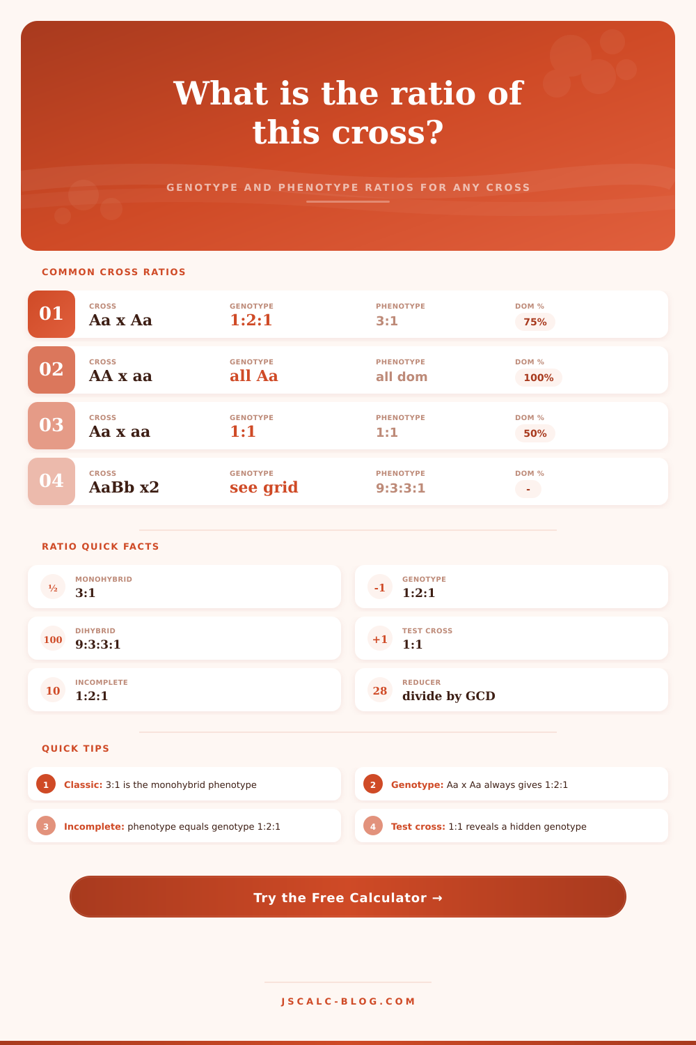
| Monohybrid | Aa × Aa | 1:2:1 | 3:1 | 75% |
| Homozygous | AA × aa | all Aa | all dominant | 100% |
| Test cross | Aa × aa | 1:1 | 1:1 | 50% |
| Back to dominant | Aa × AA | 1:1 | all dominant | 100% |
| Dihybrid | AaBb × AaBb | 1:2:1:2:4:2:1:2:1 | 9:3:3:1 | – |
| Dihybrid test | AaBb × aabb | 1:1:1:1 | 1:1:1:1 | – |
| Incomplete mono | Rr × Rr | 1:2:1 | 1:2:1 | – |
| Codominant mono | CᴿCᵂ self | 1:2:1 | 1:2:1 | – |
🔬Genotype vs Phenotype Ratios
| Parents | Genotype Classes | Genotype Ratio | Phenotype Classes | Phenotype Ratio |
|---|---|---|---|---|
| Aa × Aa | AA, Aa, aa | 1:2:1 | dom, rec | 3:1 |
| Aa × aa | Aa, aa | 1:1 | dom, rec | 1:1 |
| AA × Aa | AA, Aa | 1:1 | dom only | 1:0 |
| AA × AA | AA | 1 | dom only | 1:0 |
| aa × aa | aa | 1 | rec only | 0:1 |
| AaBb self | 9 classes | 1:2:1:2:4:2:1:2:1 | 4 classes | 9:3:3:1 |
🧪Dominance Types
| Type | Heterozygote Looks Like | Mono Phenotype | Matches Genotype? | Example Trait |
|---|---|---|---|---|
| Complete | Dominant allele only | 3:1 | No | Pea seed shape |
| Incomplete | Blended intermediate | 1:2:1 | Yes | Snapdragon pink |
| Codominance | Both alleles shown | 1:2:1 | Yes | Roan cattle coat |
| Homozygous cross | Uniform F1 | all one class | Yes | True-breeding line |
⚙How The Ratio Is Built
📋Ratio Meanings
| Ratio | Where It Appears | What It Tells You | Fraction Form |
|---|---|---|---|
| 3:1 | Aa × Aa phenotype | Three dominant to one recessive | 3/4 and 1/4 |
| 1:2:1 | Aa × Aa genotype | AA to Aa to aa proportions | 1/4, 1/2, 1/4 |
| 1:1 | Test cross Aa × aa | Even split of two classes | 1/2 and 1/2 |
| 9:3:3:1 | AaBb self phenotype | Two-trait dominant mix | 9/16 down to 1/16 |
| 1:1:1:1 | Dihybrid test cross | Four equal trait combos | 1/4 each |
💡Ratio Reading Tips
If you took biology in high school, I’m sure you recall the frustrating Punnett square: a drab grid of letters that you was supposed to fill in by hand. It was a patience exercise rather than an insight one, since you would count your alleles for minutes only to come up with a number you might’ve guessed if you’d thought about it for a second.
This page’s tool flips that script, removing the tedium of arithmetic so that you can focus on what those numbers mean biologically. Rather than spend time filling boxes in, you simply specify which parents are involved and their dominance modes, then let system do the rest. It is a tiny change in workflow but one that makes a difference because it reduces friction between wondering and knowing.
Why You Need This Punnett Square Tool
From there, it ask for the number of genes, which tells you if it is a dihybrid (examining two independent traits) or a monohybrid (examining just one, like pea color). Each extra gene increase the potential gamete combinations by 2x. So, whereas a monohybrid cross can be represented as a simple four-box grid, a dihybrid cross require a sixteen-box grid.
Most students gets stuck here, not because math is any different, but because it’s easy to mess up when you’re trying to count things manually. The calculator guarantees that all possibilities is covered and counted correctly, so you have a firm basis based off which to make your conclusions.
The math is cool, but the real lesson here lie in understanding genotype-phenotype ratios. Phenotypes are what we see, like an individual with blue eyes or brown eyes. A genotype represent the underlying genetics, such as being heterozygous or homozygous dominant.
If you do a regular cross of two heterozygous parents, the phenotypic ratio is 3:1 (under conditions of complete dominance), but the genotypic ratio is 1:2:1. Why? Homozygous dominants will appears the same as heterozygous ones. The calculator breaks those out for you so that you can see which offspring carry the recessive gene but don’t express it.
This is important if you want to predict whether someone will be a carrier of a disease or how to breed livestock on a farm. There’s also a dominance mode selector, which further increase the biological accuracy.
Many basic examples are based off full-blown dominance, where one allele completely hides the other. But nature isn’t always so simple. For example, incomplete dominance results in mixed traits. Mixing white and red snapdragons results in pink offspring.
In codominance, both alleles displays together. Examples include human blood types and the presence of roan coats in cattle. Toggle the dominance mode on those calculators and the phenotypic ratio will update to match the same 1:2:1 genotypic ratio.
This reflects an important fact about genetics: what you see depends only on how the resulting proteins interact at molecular level. Understanding this can help avoid a frequent error of using the 3:1 rule in places where it doesn’t apply.
One of the go-to methods to check for an unknown genotype is still test crosses. If you cross an unknown genotype (but dominant phenotype) individual with a homozygous recessive one, the pattern of offspring will tell you what your hidden alleles are.
If all offspring are dominant, it means the parent was homozygous; if you get a 1:1 phenotypic ratio, it were heterozygous. It takes a lot of offspring to make this approach statistically significant, so that’s why it gives you raw counts as well as simplified ratios.
Looking at actual number makes it easier to remember that those ratios are probabilities (nothing more), nothing less, and could of guarantee anything in small families. You should of used larger sample size for better accuracy.
All of these is ultimately just bridges, from the laws of Mendel to messy reality. They’re a tidy mathematical system for comparison against real-life observations. If your garden doesn’t produce the ratios the calculator says it should, well, now you know what normal is and have something to compare it to so you can understand why.
Is it that some genes aren’t separating cleanly because they’re linked? Or did random play out on a small scale? Without knowing what the normal ratio is, you don’t know what questions to ask about deviation.
It makes a chart that might otherwise seem static into a dynamic diagnostic instrument. From letters on a page, you get a closer look at the movement of traits across generations.