Linear Regression Calculator: Least-Squares Line, r, R^2

Linear Regression Calculator

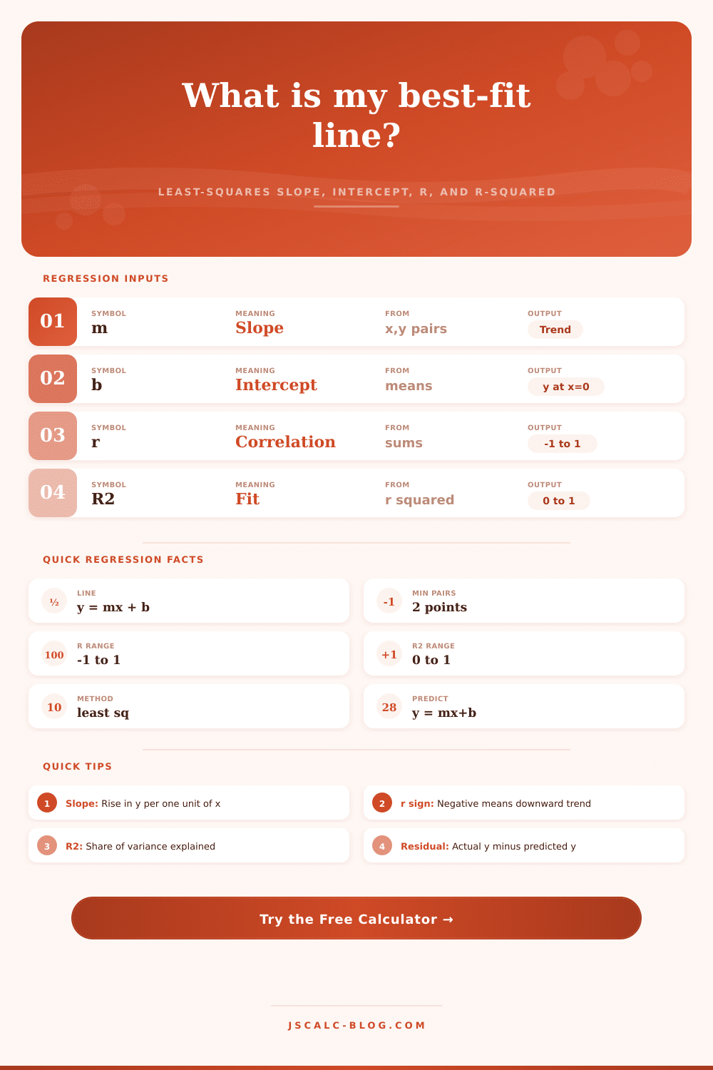
Fit the least-squares best-fit line y = mx + b to your paired (x, y) data. Get the slope, intercept, correlation coefficient r, R-squared, a full computation table, residuals, and a predicted Y for any X you choose.

📈Real Data Presets

📝Enter Your (x, y) Data

X values (independent) – comma, space, or new line separated

The predictor variable. Example: study hours, temperature, ad spend.

Y values (dependent) – must match the count of X

The outcome variable. Each Y pairs with the X in the same position.

Predict Y at this X value

Estimates y-hat = m × X + b at your chosen X.

Decimal places

Row order for tables

Residuals table

Fourth result card shows

Best-fit equation y = mx + b least-squares line

Slope (m) 0 change in y per unit x

Correlation (r) 0 strength and direction

R-squared 0 variance explained

🔢Formula Snapshot

nData pairs

mSlope

bIntercept

R²r squared

🧮Least-Squares Computation Table

#	x	y	x × y	x²	y²
Enter X and Y data above to build the computation table.

📏Residuals Table

#	x	y actual	y predicted	residual	residual²
Residuals appear after calculation.

📊Correlation Strength Reference

\|r\| Range	Strength	R-squared Range	Interpretation
0.90 – 1.00	Very strong	0.81 – 1.00	Points hug the line; predictions are reliable
0.70 – 0.89	Strong	0.49 – 0.79	Clear trend with modest scatter around the line
0.40 – 0.69	Moderate	0.16 – 0.47	Real but loose relationship; use with caution
0.20 – 0.39	Weak	0.04 – 0.15	Faint pattern; the line explains little variance
0.00 – 0.19	Negligible	0.00 – 0.03	Essentially no linear link between x and y

🗂Regression Scenario Comparison

Scenario	X Variable	Y Variable	Expected Slope	Typical r	Use Case
Study time	Hours studied	Exam score	Positive	0.85 to 0.95	Predict grades from effort
Retail seasonality	Temperature	Cold drink sales	Positive	0.80 to 0.97	Plan inventory by weather
Growth chart	Height	Weight	Positive	0.70 to 0.90	Screen for healthy ranges
Marketing	Ad spend	Revenue	Positive	0.60 to 0.90	Estimate return on spend
Economics	Price	Quantity demanded	Negative	-0.70 to -0.95	Model a demand curve
Careers	Years experience	Salary	Positive	0.65 to 0.90	Benchmark pay by tenure

⚙Full Formula Breakdown

Data pairsEach observation is a pair (x, y). You need at least 2 valid pairs and X values that are not all identical.

Required sumsSx = Σx, Sy = Σy, Sxy = Σ(x×y), Sxx = Σx², Syy = Σy², over all n pairs.

Slope mm = (n·Sxy – Sx·Sy) / (n·Sxx – Sx²). It is the rise in y for a one-unit rise in x.

Intercept bb = (Sy – m·Sx) / n. This is the predicted y when x = 0, and the line passes through the point (mean x, mean y).

Correlation rr = (n·Sxy – Sx·Sy) / √((n·Sxx – Sx²)·(n·Syy – Sy²)). It ranges from –1 to +1.

R-squaredR² = r². It is the share of the variance in y that the fitted line explains, from 0 to 1.

PredictionFor any X, the predicted value is y-hat = m×X + b. The residual for a point is y – y-hat.

📘Regression Terms Glossary

Term	Symbol	Meaning	Range or Units
Slope	m	Steepness of the fitted line	Any real number
Intercept	b	Predicted y when x = 0	Any real number
Correlation	r	Strength and direction of linear link	–1 to +1
Coefficient of determination	R²	Variance in y explained by the line	0 to 1
Predicted value	y-hat	Estimate from the line at a given x	Same units as y
Residual	e	Actual y minus predicted y	Same units as y
Sum of squared residuals	SSE	Total squared prediction error	Minimized by least squares

💡Practical Regression Tips

Correlation vs cause: A high r shows x and y move together, not that one causes the other. A hidden third variable can drive both, so confirm the mechanism before acting.

Mind the range: The line is only trustworthy near the x values you measured. Predicting far outside that range (extrapolation) can give misleading y-hat values.

You have some numbers paired together (like ad spending vs. Revenue) or other things like time studied vs. It is a test score. And you want to know if there’s a pattern in the data.

Well, linear regression can help you figure out that pattern. Not magic, mind you, just pretty good for most practical applications. It fits a line to your data so that the sum of squares of differences between observed points and predicted values is minimized. This is known as least-squares line. It also provides an equation describing relationship between one variable and another.

What Is Linear Regression?

From this, you derive the slope and intercept. The former indicate how fast the variable changes; the latter pins down where on the x-axis the line hits the y-axis. But the true value is knowing what these numbers tell you about your own circumstance.

But slope, how much one variable change for every one-unit change in the other, is usually the simplest to grasp. More study time? Better grades? That’s the expectation with a positive slope. But a negative slope reverses everything. Price down = Demand up? Those are healthy signs in any economy. Your job is to know how to interpret the direction, something the calculator figure out from the algebra for you. One mistake people make all the time here: they get the sign backward and draw incorrect conclusions.

And then there’s r, or the correlation coefficient. This represents the degree to which points group along best-fit line. R can range between -1 to 1. It doesn’t say whether one thing causes another; it indicates that when this happens, that also happens. And that difference matter much more than many think. Both shark attacks and ice cream sales increase in July, for instance, but sharks don’t flock for cones.

(The page has a handy chart classifying correlations by strength, and a reminder that even with a weak correlation, you explain only a small amount of the variance in your results.) That’s where R-squared comes into play. It extends that correlation with a measure of explained variance as a percent. So if an R-squared is one, it’s a perfect fit (with all points lying on the curve), and if it’s zero, it’s completely useless for predicting anything. In reality, most business data don’t look like that. The trend is there, but it’s muddied by other factors, and most business metric hover somewhere in the middle, moderately predicted. What matters then is not just understanding the trend itself, but knowing what kind of error to anticipate… So you can have confidence in your prediction.

You’ll notice the error spelled out in form of residuals. Residuals are simply the difference between what the model predicted and what actualy occurred. These should appears random with no obvious patterns present. This indicates a good model. Perhaps the linear assumption was incorrect from the beginning if you observe a pattern (e.g., a curve) when looking at the residuals. You can check for this by inspecting the residual table. It’s worth taking a moment to go through it… Don’t just glance at the final equation.

In most cases, it’s all about prediction. With the line, you’re able to predict a Y value given a new X input. Within your range of initial data points, that works fine. But if you guess way out into places where you haven’t seen anything happen, where the trend bends and breaks at extremes… That becomes dicey. You can put a particular X value into the tool and get an estimate of how it would of work. That’s useful for rapid scenario planning.

Linear regression boils down complexity while keeping its truth. You get a line through a cloudy dot plot. Clarity from scatter. It is a tool for spotting trends, checking assumptions, and making an educated guess. But remember: it’s just a line. It is a moddern model, not a law of nature. All the messy details remain in the data, none of which any equation can ever fully include.