Least Squares Regression Line Calculator (y = mx + b)

Least Squares Regression Line Calculator

Fit the best straight line y = mx + b to paired data using the least squares normal equations. See the running sums, the slope and intercept computation, R-squared, residuals, the minimized sum of squared errors, and a prediction for any x value.

📈Real Data Presets

📝Paired Data & Options

X values (independent, comma or space or newline separated)

The predictor variable. Each X must have a matching Y in the same position.

Y values (dependent, same count and order as X)

The response variable you want the line to predict.

Slope method shown first

Predict Y at X =

Plugs this X into y-hat = mx + b for a point estimate.

Decimal places

Computation table (x, y, xy, x²)

Residuals table (y – y-hat)

Max data rows displayed

Regression line y = mx + b least squares best fit

Slope (m) 0 change in y per unit x

Y-intercept (b) 0 value of y when x = 0

R-squared 0 share of variance explained

🔢Key Quantities

0Pairs (n)

0Mean of x

0Mean of y

0Correlation r

📊Computation Table (Sums for the Normal Equations)

#	x	y	x × y	x²	y²
Enter paired data above to build the computation table.

📏Deviation Score Table (About the Mean)

#	x – x̄	y – ȳ	(x–x̄)(y–ȳ)	(x–x̄)²	(y–ȳ)²
Deviation scores appear here after calculation.

🔍Residuals & Minimized Error

#	x	y	y-hat = mx+b	Residual (y – y-hat)	Residual²
The residuals table appears after calculation.

📐Regression Line Interpretation

Element	Value	What It Means
Fit the line to see a plain-language interpretation.

🎯Goodness of Fit Snapshot

Measure	Symbol	Value	Reading
Goodness-of-fit measures appear after calculation.

🗂R-squared Strength Reference

R-squared Band	r Range	Fit Strength	Points Near Line	Prediction Trust
0.90 to 1.00	0.95 to 1.00	Very strong linear	Very tight	High
0.70 to 0.90	0.84 to 0.95	Strong linear	Close	Good
0.50 to 0.70	0.71 to 0.84	Moderate linear	Some spread	Fair
0.30 to 0.50	0.55 to 0.71	Weak linear	Loose cloud	Low
0.10 to 0.30	0.32 to 0.55	Very weak	Wide scatter	Very low
0.00 to 0.10	0.00 to 0.32	No linear pattern	Random cloud	Not usable

⚙Full Formula Breakdown

GoalFind the line y = mx + b that minimizes SSE = sum of (y – y-hat)², the total squared vertical distance from each point to the line.

Running sumsFrom n paired points compute Sx, Sy, Sxy, Sxx, Syy, where Sxy = sum(x×y), Sxx = sum(x²), Syy = sum(y²).

Slope (normal eq)m = (n×Sxy – Sx×Sy) / (n×Sxx – Sx²). This solves the least squares normal equations for m.

Slope (deviation)m = SSxy / SSxx where SSxy = sum((x–x̄)(y–ȳ)) and SSxx = sum((x–x̄)²). Same slope, different form.

Interceptb = (Sy – m×Sx) / n = ȳ – m×x̄. The fitted line always passes through the mean point (x̄, ȳ).

Correlationr = (n×Sxy – Sx×Sy) / sqrt((n×Sxx – Sx²)(n×Syy – Sy²)). It shares its sign with the slope.

R-squaredR² = r² = 1 – SSE / SST, where SST = sum((y–ȳ)²). It is the share of y variation explained by the line.

PredictionFor any x, the fitted value is y-hat = m×x + b. Best used inside the observed range of x (interpolation).

📋Reference Values

Symbol	Name	How It Is Built	Role in the Line
n	Sample size	Count of paired points	Scales every sum
Sxy	Sum of products	sum(x × y)	Numerator of slope
Sxx	Sum of x squares	sum(x²)	Denominator of slope
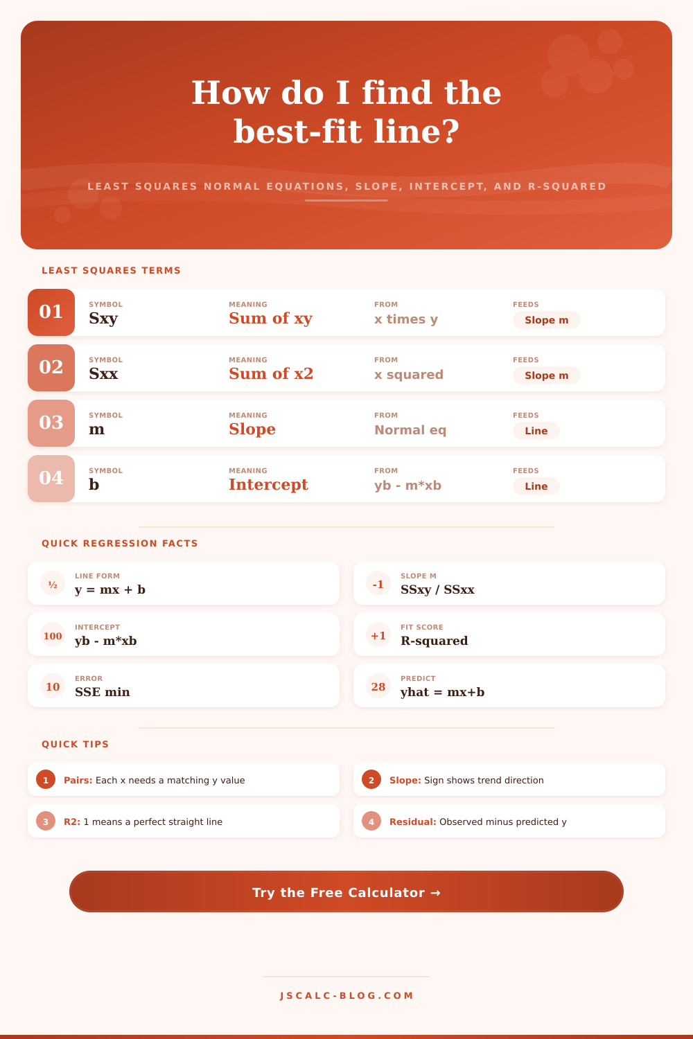
m	Slope	SSxy / SSxx	Tilt of the line
b	Intercept	ȳ – m×x̄	Height at x = 0
SSE	Squared error	sum((y – y-hat)²)	Quantity minimized

💡Least Squares Tips

Why squared errors: Squaring the residuals makes every miss positive and penalizes big gaps more than small ones, so the line settles where the total squared vertical distance is smallest.

Predict with care: The slope and intercept describe the data you supplied. Predicting far outside the observed x range is extrapolation and can drift well away from reality.

It’s your scatter plot: a collection of points standing before you as if someone dumped a bag of gravel onto a sheet of graph paper. There are no clear answer. It is just a mess of information and a reluctance to give up any clue. But maybe there is something beneath that noise. Maybe more time spent studying does result in better test grade. Maybe ad dollars do in fact increase sales. And that’s when the least squares regression line calculator helps us find a pattern in the mess.

This is a straight line running through the mess. It doesn’t simply assume where the pattern lies, but instead use math to force data to show its clearest linear signal at point of minimum total squared error.

How Least Squares Regression Works

You provide a pair of numbers (one for Y and another for X). It doesn’t matter which is which (though it does if you want calculator to function). Each number on one row should match only with the corresponding number on other row. Mess them around, and the whole thing falls apart like house of cards.

Next, the calculator derives two key elements: the intercept and the slope. The slope describes both how steeply related the two variable are and in what direction. Positive slope? Your two variables is going in the same direction. Negative slope? They’re inversely related, meaning that when one increases, the other decrease. How much? That’s the magnitude.

The intercept is frequentlly misinterpreted as a real-world point. It’s not; it’s a theoretical one that in most real-world situation does not exist at all. What it refers to is the Y value at which X = 0. While in many practical scenarios this number is useless for prediction, it is still essential for positioning the line correctly across your actual data range.

The algorithm force the fitted line to pass through the mean of both X and Y. That’s its anchor point, and it assures a balanced result. The sum of residuals above the line will always be exactly equal to the sum of residuals below the line.

The typical decision point for keeping a model or throwing it out, however, is R-squared, which is measure of how well your independent variable explain the variation in your dependent variable. The closer to one, the tighter the fit, with points hugging the line more closely. The closer to zero, the less predictive the line and the more sense it make to guess at the average.

The reference table on the page helps you quickly understand what these bands mean without having to remember statistical thresholds.

A key point to note here is exactly what the calculator aim to minimize. Specifically, it minimizes the sum of squared errors. Residuals are squared, so the larger the error, the higher the penalty. That’s good because it ensures that one huge outlier won’t be overlooked and little wiggles will go unnoticed. As such, you end up with a line that hugs the thickest portion of the cloud. But it also make it so that even a few really extreme outliers can throw off results.

Extrapolation! Beware: this thing only knows what you’ve fed to it. It’s dangerous to predict values that is much farther from what you observed in X area. What works in small quantities may plateau or even curve at larger sizes. Don’t expect this kind of linearity, and even if the calculator spits out a number, don’t assume you can trust it. You need judgment beyond the math. Be sure to verify that your prediction is in the domain of known data.

The breakdown sections shows how to calculate the slope in two ways: one with raw numbers (sums of products, etc.), and another with deviations from the mean. Each arrive at the same result but provides a slightly different perspective on the calculation itself. Seeing both should make it clear where each part comes from as they combine into an equation. Regression isn’t magic, after all; it’s a matter of accounting for distance, systematically.

To summarize: The best-fit line is just about imposing order on randomness. It’s the one straight line that stays as close as possible to every individual point vertically. With that in mind, and when you respect the limits of guessing, the tool acts as a powerful lens through which to view patterns. That gravel spill begins to stop appearing as noise and more like a signal.