Confidence Interval Calculator
Build a confidence interval for a population mean or a proportion using the z score or Student t distribution. See the critical value, standard error, margin of error, and the full low-to-high interval with every step shown.
🎯Real Scenario Presets
📝Interval Inputs
Used only when level is set to custom. Between 50 and 99.99.
Standard deviation of the whole population.
Standard deviation from your sample data.
Enter as a decimal, for example 0.52 for 52%.
Applied only when the correction is on and N is finite.
🔢Formula Snapshot
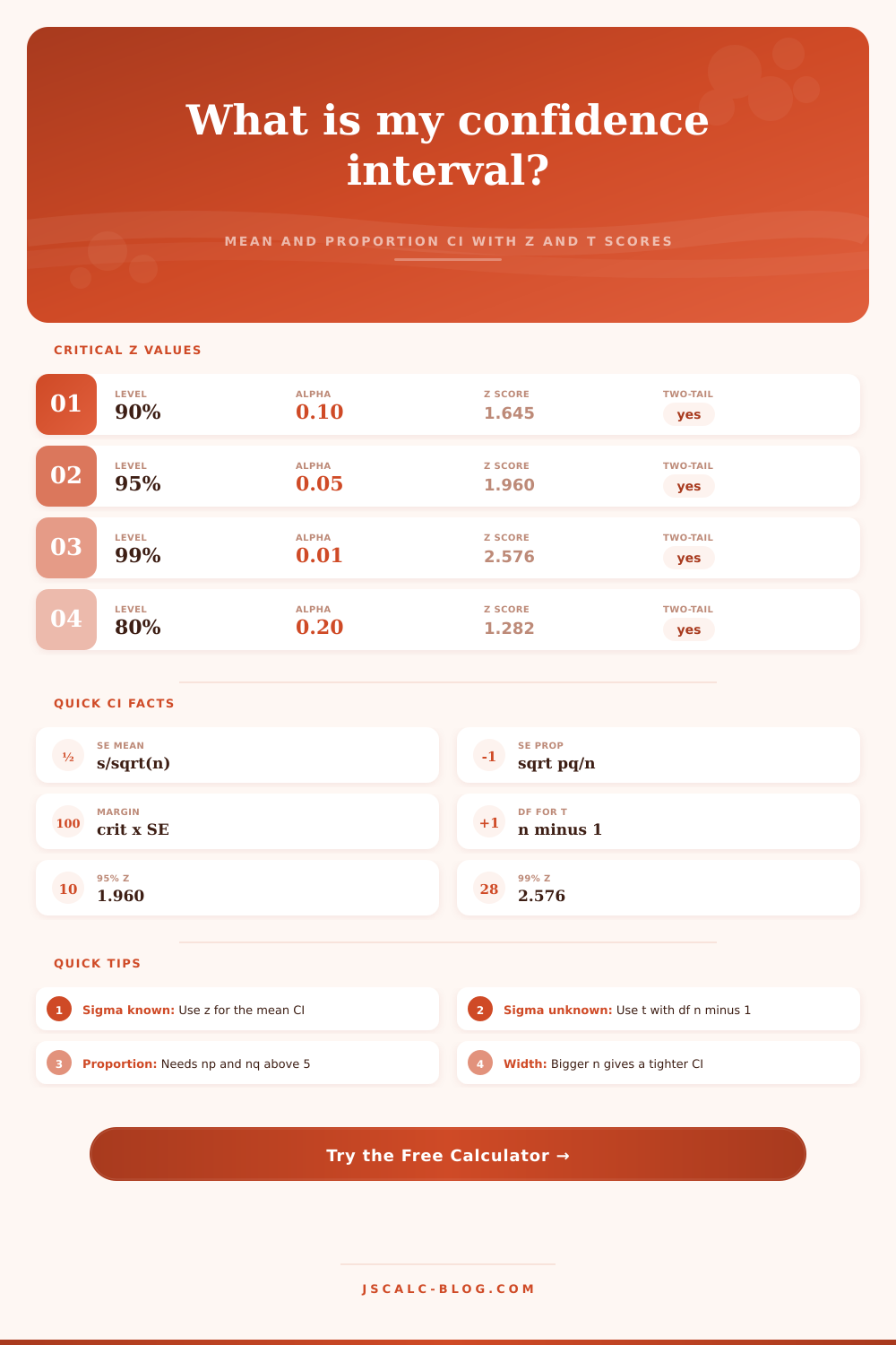
📊Critical z Values
| Confidence | Alpha | Alpha / 2 | Two-Tail z | One-Tail z |
|---|---|---|---|---|
| 80% | 0.20 | 0.100 | 1.282 | 0.842 |
| 85% | 0.15 | 0.075 | 1.440 | 1.036 |
| 90% | 0.10 | 0.050 | 1.645 | 1.282 |
| 95% | 0.05 | 0.025 | 1.960 | 1.645 |
| 98% | 0.02 | 0.010 | 2.326 | 2.054 |
| 99% | 0.01 | 0.005 | 2.576 | 2.326 |
| 99.9% | 0.001 | 0.0005 | 3.291 | 3.090 |
📈Critical t Values (Two-Tail)
| df | Sample n | 90% t | 95% t | 99% t |
|---|---|---|---|---|
| 1 | 2 | 6.314 | 12.706 | 63.657 |
| 4 | 5 | 2.132 | 2.776 | 4.604 |
| 9 | 10 | 1.833 | 2.262 | 3.250 |
| 14 | 15 | 1.761 | 2.145 | 2.977 |
| 19 | 20 | 1.729 | 2.093 | 2.861 |
| 24 | 25 | 1.711 | 2.064 | 2.797 |
| 29 | 30 | 1.699 | 2.045 | 2.756 |
| 49 | 50 | 1.677 | 2.010 | 2.680 |
| 99 | 100 | 1.660 | 1.984 | 2.626 |
| ∞ | large | 1.645 | 1.960 | 2.576 |
🗂Method Comparison Grid
| Method | Use When | Standard Error | Critical | Interval | Notes |
|---|---|---|---|---|---|
| Mean z | Sigma known or n large | sigma / sqrt(n) | z | xbar ± E | Normal model |
| Mean t | Sigma unknown, use s | s / sqrt(n) | t, df n–1 | xbar ± E | Wider than z |
| Proportion z | Count or percent data | sqrt(pq / n) | z | p ± E | Wald interval |
| Small mean | n under 30, s only | s / sqrt(n) | t | xbar ± E | Assumes normal |
| Large poll | n over 1000 percent | sqrt(pq / n) | z | p ± E | Tight margin |
| Finite pop | Sample near N size | SE × FPC | z or t | est ± E | Shrinks SE |
⚙Full Formula Breakdown
📋Margin of Error Reference
| Item | Typical Range | Effect on Interval | Why |
|---|---|---|---|
| Confidence level | 90% to 99% | Higher level, wider CI | Larger critical value |
| Sample size n | 10 to 5000 | Larger n, tighter CI | SE falls with sqrt(n) |
| Spread (s or sigma) | Data dependent | More spread, wider CI | SE grows with spread |
| Proportion near 0.5 | 0 to 1 | Widest at p = 0.5 | p(1–p) is maximal |
| z versus t | Small n | t gives a wider CI | Heavier t tails |
💡Practical CI Tips
Uncertainty comes in form of confidence intervals: a range within which it’s likely that true number lies given our small amount of data. The plus or minus three points on a poller saying “52% support” means actual number is probably somewhere between 49 and 55 percent. It is not one thing, but a recognition that we don’t have the exact value for population parameter.
How do you calculate this range? You use z-score or a t-score. If you pick the right option in calculator, it’ll make that decision for you. Under what circumstances should you use a z-distribution instead of a t-distribution? You should use it only if you have access to population standard deviation (which is rare outside of textbook problems). Most of the time you’re estimating that spread based off some sample data.
Understanding Confidence Intervals
The t-curve has fatter tails than normal bell curve. That takes into account the added uncertainty involved with estimating the standard deviation from a small number of observations. That becomes important when your sample size is small. Otherwise, you could wind up with an interval too tight because you used z-score. By contrast, the t-score widens net and keeps you honest.
That net gets wider pretty quickly depending upon which confidence level you choose. You want 99% confidence? Then you’d better make it wide enough to account for way more possibilities. But 90%? It is not so bad. It’s an intuitive trade-off.
You want to know whether or not your method is reliable enough to capture the true parameter, but remember that a 95% confidence interval doesn’t actually mean there’s a 95% chance the parameter is in that specific range. Check out table of critical values on this page. Notice how much the multiplier jumps from 90% confidence (z = 1.645) to 99% confidence (z = 2.576). The bigger number widens your interval considerably. Statistics isn’t broken. It’s expensive to get more certain.
The real lever you have control over is sample size. As your sample increases, the standard error decreases slowly because of its square root relationship. For example, doubling your sample only cuts down the standard error by roughly 41%. This diminishing return throws researchers for a loop. They’d like tighter precision, so they double their sample and expect half the margin of error. Never gonna happen. To cut width of your interval in half, you need four times the amount of data.
It is expensive and slow, which is why you’ll frequently find surveys settling on a sample size of a thousand, no matter if population is ten thousand or ten million. Once your sample gets big enough relative to the population, the math don’t care how big the population is. But it gets interesting in terms of proportion when your guess is around 50%. That’s the point of maximum uncertainty: there’s more room for a split vote than there is for a landslide. The standard error formula use the product of p times q. When both are half, that product is as large as possible.
Plan your study to account for worst-case variance (at 50%) so that your sample size will be sufficient even if actual proportion differs from what you think. Better safe than sorry: it’s better to over-estimate than realize afterwards that your confidence interval is too wide to provide any guidance.
When your sample represents a substantial portion of overall population there’s also the matter of a finite population correction factor: if you’re surveying from staff of 100, and you’re polling 50, then standard formulas don’t apply, as they assume an infinite pool. Since you’ve already encountered half the population, that correction narrows the interval. You know more than the standard model knows. It’s a small adjustment, but important for quality control checks and internal audits where N isn’t huge.
Now we come to the last hurdle: interpreting result. The 95% confidence interval is not saying that there’s a 95% chance parameter falls within this particular interval. There is no probability assigned to the parameter! It either is or it isn’t. The 95% is a statement about the process. If I ran this study thousands of times, 95% of these computed intervals will include the true value.
This confuses both student and execs. We want a probabilistic statement about a single result. But frequentist statistics doesn’t provide this directly. It provides reliability of the process. You get to see how it’s calculating the width for each step (standard error to final bounds), which I think is helpful.
So next time you’re looking at customer satisfaction scores or trying to analyze results of a medical trial, now you know the math behind it all and won’t be tricked into thinking your sample size is representative when it probably isn’t. Margin of error isn’t something to hide. It’s the cost of working with imperfect information. Build the interval. Check the assumptions. Accept that truth is probably within this range, although we don’t know precisely where. You should of used a larger sample for more accuratley results.