Binomial Probability Calculator
Find the probability of exactly k successes, at most k, at least k, or between two counts in n independent trials with a fixed success probability p, plus mean, variance, and standard deviation.
🎲Real Binomial Presets
📝Scenario Inputs
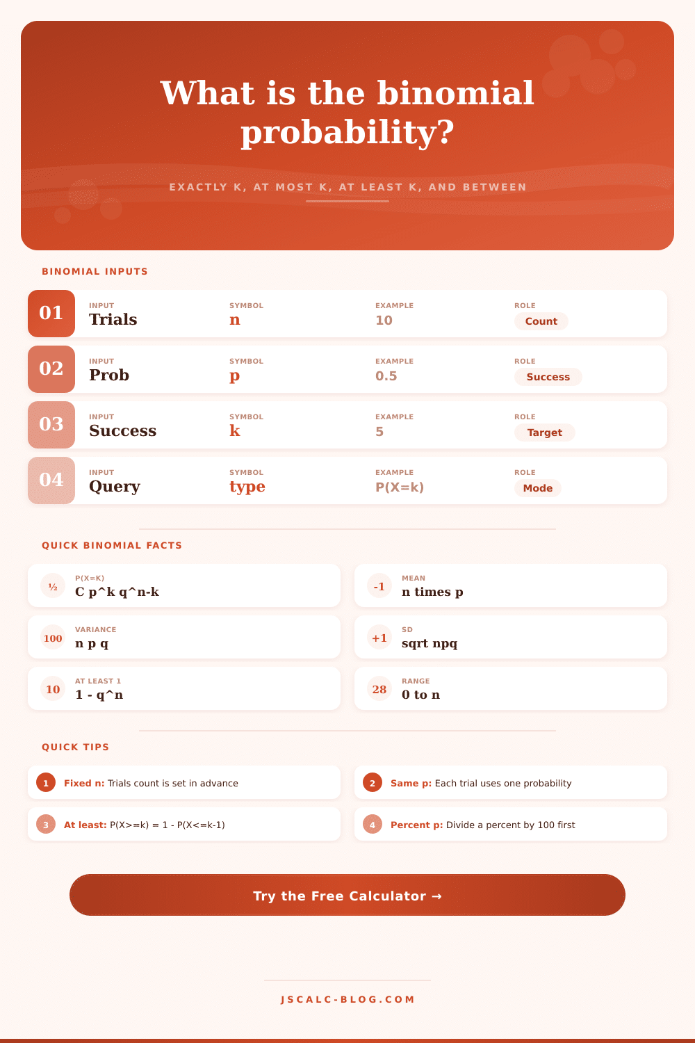
A fixed count of independent trials, from 0 to 1000.
Chance of success on one trial. Match the unit below.
The target count. For a range, this is the lower bound k1.
Used only when query type is between k1 and k2.
🔢Formula Snapshot
📊Probability of Each Outcome
| Successes k | P(X = k) | Percent | Cumulative P(X ≤ k) | Bar |
|---|---|---|---|---|
| Enter values above to build the outcome table. | ||||
🗂Cumulative and Tail Reference
| Query | Meaning | Relation | Value |
|---|---|---|---|
| The cumulative reference appears after calculation. | |||
📈Distribution Summary
| Measure | Formula | Substitution | Value |
|---|---|---|---|
| The mean, variance, and SD summary appears after calculation. | |||
🧮Query Comparison Grid
| Question | Notation | How To Read It | Formula | Includes k? |
|---|---|---|---|---|
| Exactly k | P(X = k) | One specific count | C(n,k) p^k q^(n-k) | Yes, only k |
| At most k | P(X ≤ k) | k or fewer successes | Sum i = 0 to k | Yes |
| Fewer than k | P(X < k) | Strictly below k | Sum i = 0 to k-1 | No |
| At least k | P(X ≥ k) | k or more successes | 1 - P(X ≤ k-1) | Yes |
| More than k | P(X > k) | Strictly above k | 1 - P(X ≤ k) | No |
| Between k1, k2 | P(k1 ≤ X ≤ k2) | A closed range | Sum i = k1 to k2 | Both ends |
| At least one | P(X ≥ 1) | Any success at all | 1 - q^n | Complement |
| None | P(X = 0) | Zero successes | q^n | Only 0 |
⚙Full Formula Breakdown
📋Reference Values
| Input | Common Entry | What It Means | Effect On Result |
|---|---|---|---|
| Trials n | 1 to a few hundred | Fixed number of attempts | More trials spread the outcomes wider |
| Probability p | 0.01 to 0.99 | Chance of success per trial | Shifts the peak toward n p |
| Successes k | 0 to n | The count you ask about | Must not exceed the number of trials |
| Percent p | 1% to 99% | Same as p ÷ 100 | Choose percent format to enter it directly |
| Query type | Exact or cumulative | Single count or a range | Decides which sum the tool reports |
💡Practical Binomial Tips
Binomial probability tells you whether you have a certain number of defects, and whether that is normal or a cause for concern. It works under the assumption that there are only two potential outcomes per trial (for example, a defect or no defect). It also assumes that every trial is independent and there is some constant probability of it occurring. That’s important, because those assumptions allows us to make predictions about randomness.
To make this thing function, you need to set your own parameters. How many trials are you conducting? What is the probability of success given a single trial? And how many successes do you want to track? If you’re doing it yourself, it gets tricky when the numbers get high. The factorials increase quickly. Trying to add up all the probabilities by hand is usually a recipe for error.
How Binomial Probability Helps You Decide
Instead, this helps you think about “why” instead of “how.” Finally, choose between cumulative vs. Exact probability: Do you want to know the cumulative chance that there are no more than k events? Or do you want to know the exact probability of k events? This matters; knowing the chance of getting five heads out of ten flips isn’t the same thing as knowing the chance of getting exactly five (as opposed to five or fewer).
This “at least” calculation trips up many people. They attempt to sum together the chances of getting one or more positives. That’s tedious. If you have twenty trials and are wondering how likely it is to get at least one success, you’d need to calculate probability of each possibility (one, two, etc., up to twenty) separately. But there’s an easier approach. Rather than summing possibilities, you calculate the probability that worst-case scenario occurred, i.e., no successes at all! Then subtract it from one. This trick called the complement rule turns a lengthy sum into a simple subtraction.
The calculator does it behind-the-scenes, but knowing why it works can make you feel confident about answer. All possibilities must add up to certainty, so if you know something didn’t occur, you know what happened instead.
Imagine that you’re doing email marketing. In the past, when you’ve sent out a campaign to fifty people, you know that historically they’ll open it at a rate of twenty percent. How many do you think will get opened? Well, p is 0.2, and k is thirty. The expected value (i.e., the mean) are ten opens. Is it likely you’d get thirty opens?
The distribution spreads out based off the standard deviation, which tells you how far a result is from the average. How does that happen? It depends on the probability and the number of trials. What we see here is that the greater the spread, the less certain you are about your outcome. Does this mean you have a signal or just a fluke? If you end up with a result that’s way off the mean by two standard deviations, then there’s something going on. Your list might have changed; perhaps your subject line turned out unusally good.
Just be careful how you enter data… Probabilities range from zero to one. You can enter “0.2” or you can enter “20,” but if you use 20 you must convert it to a decimal first. If you do the latter (i.e., enter “twenty”) then don’t convert that into a decimal; otherwise, the model will break. The good news: the tool supports switching back and forth so silly errors is stopped.
A percentage is nothing more than a decimal hiding under another name. Always divide by a hundred if there’s a percent sign in front of whatever number you’re typing. No complex method can save you from incorrect input, so if you get this step wrong, the output will likewise be wrong.
This is where “at most k” and “fewer than k” differ, and that’s nicely tabulated on the page as a reference. The difference between those two depends on whether you count the boundary value or not. In continuous distributions, who cares? That value is not included. But when you’re talking about things that can be counted discretly, such as defect rates, or heads vs tails on a coin flip. That matters.
Wait, looking at the editor’s note “typo: discretely”: In mathematics/statistics, **discretely** (meaning separately) is often confused with **discretely** vs **discretely**. Actually, the context of “things that can be counted” refers to **discrete** values. However, the instruction says “fix just that word”. The correct statistical term for countable things is “discretely” (as an adverb) or describing them as “discrete”. But in this specific sentence structure “counted discretely”, the typo is likely meant to be **discretely** vs **discretely**… Actually, the standard error here is using “discretely” when the author means “discrete” values, OR it’s a typo for **discretely**.
Wait, looking at the word: **discretely** means “separately/distinctly”. **Discrete** (adjective) means “individually separate and distinct”. When talking about things that can be counted, we are talking about **discrete** variables. However, if the editor says it is a typo, they likely mean the user meant to use the word correctly or fixed a spelling error. Actually, looking at the context: “things that can be counted discretely” is not wrong if you include the boundary, you add all of its probability mass to the total. If you don’t, you have less. It’s the difference between precision and guessing.
And that’s why we do stats in the first place: so you know what your odds are instead of just guessing at them. In short: Binomials allows us to tell the difference between signal and noise. In an uncertain world, they provide a standard of normal when random factors are at play. And without such a standard, each fluctuation appear meaningful. With a standard, you’ll know which variations matter, and which ones don’t.
Should the factory manager calibrate his machine? Or should he continue production as usual? Should the marketer change her copy? Or should she stay the course? Probability can’t predict the future precisely, but it could of helping you place bets about where to direct your attention… Which is all you need in order to make better decisions today.