Binomial Distribution Probability Calculator + PMF Table

Binomial Distribution Calculator

Build the complete binomial distribution for n trials with success probability p: the full PMF table for every k from 0 to n, cumulative probabilities, the mean, variance, standard deviation, mode, and skewness, plus a normal-approximation check.

🎯Real Distribution Presets

📝Distribution Inputs

Number of trials n

Each trial is independent with two outcomes.

Probability entry method

Success probability p

Decimal 0 to 1, or a percent if selected above.

Highlight outcome k

Marks one row and feeds the fourth result card.

Decimal places

PMF table row cap

Large n condenses the low-probability tails.

Probability display

Fourth result card shows

Mean μ 0 expected successes = np

Std deviation σ 0 sqrt of the variance

Variance σ² 0 np(1 – p) spread

Most likely k 0 mode of the distribution

🔢Formula Symbols

nNumber of trials

pSuccess probability

kSuccesses counted

qFailure = 1 – p

📊Full PMF and Cumulative Table

k Successes	P(X = k)	P(X ≤ k)	P(X ≥ k)	Relative Bar
Enter n and p above to build the full PMF table.

📐Distribution Summary

Measure	Formula	Substitution	Value
The summary statistics appear after you build the distribution.

📈Cumulative Reference Points

Query	Meaning	Probability	Percent
Common cumulative queries appear here after calculation.

🔔Normal Approximation Check

Rule of thumbThe normal approximation is generally reliable when both np and n(1 – p) are at least 5.

🗂Distribution Shape Comparison

Scenario	n	p	Mean np	SD	Skewness	Shape
Fair coin	10	0.50	5.00	1.581	0.000	Symmetric
Survey opt-in	20	0.30	6.00	2.049	0.195	Right skew
Free throws	15	0.75	11.25	1.677	–0.298	Left skew
Defect rate	40	0.05	2.00	1.378	0.653	Strong right
Balanced survey	25	0.60	15.00	2.449	–0.082	Near normal
Quality batch	50	0.50	25.00	3.536	0.000	Bell shaped

⚙Full Formula Breakdown

PMFP(X = k) = C(n, k) × p^k × (1 – p)^(n – k), where C(n, k) is the binomial coefficient n! / (k!(n – k)!).

CoefficientC(n, k) is built iteratively as C(n, k) = C(n, k – 1) × (n – k + 1) / k to avoid huge factorials.

CumulativeP(X ≤ k) is the running sum of P(X = 0) through P(X = k); the full row set sums to 1.

Meanμ = n × p is the expected number of successes over the n trials.

Varianceσ² = n × p × (1 – p); the standard deviation σ is its square root.

ModeThe most likely outcome is floor((n + 1) × p); when (n + 1)p is an integer, two adjacent modes tie.

SkewnessSkew = (1 – 2p) / sqrt(n × p × (1 – p)); it is zero when p = 0.5 and grows as p moves toward 0 or 1.

📋Reference Values

Item	Typical Range	How It Is Used	Effect On Shape
Trials n	1 to 1000	Sets the count of PMF rows	Larger n looks more bell shaped
Probability p	0 to 1	Weights successes vs failures	p near 0.5 is symmetric
Mean np	0 to n	Centers the distribution	Marks the peak region
SD sqrt(npq)	0 to n/2	Measures the spread	Wider bars with mid p
Skewness	–∞ to ∞	Measures tail direction	Sign follows 1 – 2p

💡Practical Distribution Tips

Reading tip: The P(X = k) column gives one exact bar height, while P(X ≤ k) answers at most questions and P(X ≥ k) answers at least questions without re-summing by hand.

Shape tip: When p sits far from 0.5 the peak leans toward the closer edge, so the mode and the mean np can land on different integers even though both describe the center.

The binomial distribution apply to binary decisions, in other words, any decision with exactly two options. That’s true of quality control checks, election polls, and coin flips. It’s true of calculating likelihood that your morning commute will be delayed by a specific number of red lights.

The idea is straightforward: There are some fixed number of trials. Each trial has exactly two possible outcome. You could label them success/failure. Or you could label them heads/tails. Whatever. What makes this hard is knowing which ones to stack on top of each other.

How Binomial Distribution Works

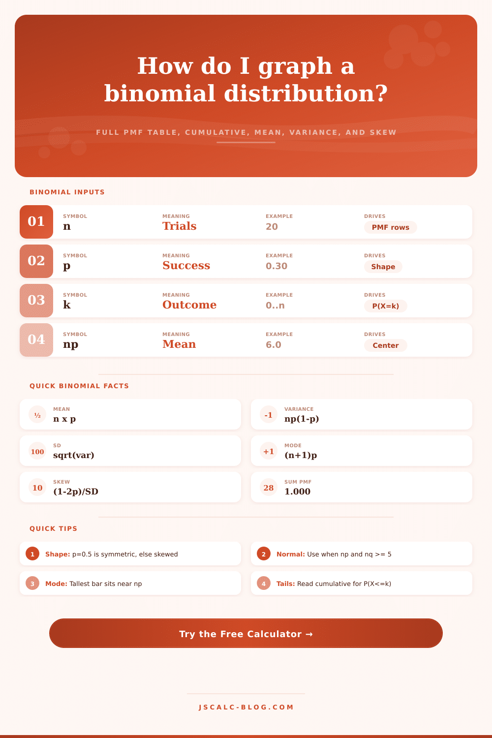
To calculate it, however, you have to define the parameters. What’s your number of trials? How many times are you going to flip that coin? That establishes the scale. Then what’s the probability of success on each trial? What’s the probability of heads coming up on any given coin toss? And there lies the thing: That parameter defines the shape of everything thereafter.

If the probability of success per trial is fifty percent, then the resulting distribution will be perfectly symmetric. It’ll form a nice, tidy bell curve right smack dab in the middle. But if the probability goes toward one or zero, then suddenly the entire structure skews. Suddenly the peak shift toward the extreme. The tail lengthens away from it.

Most folks fail to grasp this. They think randomness ought to look uniform. They don’t understand how asymmetry comes from bias.

After you input your number of trials and success rate, the calculator does all the math for you, no need to do it by hand using factorials. It outputs an entire table of probabilities. That’s a list of the precise probability of zero successes, one success, two successes, and onward. It goes all the way through to perfect results.

That’s where it gets realy useful: You can read that table. In most situations, folks just want to know their chance of hitting exactly what they’re looking for. And yet, in the real world, you’ll often care about ranges. Will at least half the survey responders say yes? Will there be fewer then three defects in the batch? Those questions have cumulative probabilities as an answer.

You don’t need to add all the rows together yourself. It computes a running total, bottom-up. That’s useful if you want to establish some threshold. Maybe you’re overseeing a production line and you’d like to know what’s the probability that more than a given number of defects will occurs. Then you can set your own safety margin based off this probability.

How closely do these outcomes group around the mean? The standard deviation help you with that. Close results are predictable, while wide results mean anything could happen. That can help you plan for the worst case.

There’s also something else worth keeping an eye out for: skewness. Skewness measures whether the distribution is lopsided. A left-skewed curve indicates that there’s a high chance of success. Extreme low results are still possible but not likely. A right-skewed curve indicate that success isn’t very probable.

Why does this matter? If skew is severe, then normal approximations won’t work. For this reason, the calculator checks to see if skew is a problem. If so, then it will alert you if your chosen probability and/or sample size result in a poor normal approximation. In other words, don’t trust general rules of thumb in these situations, but do trust the exact binomial calculation.

Inputs come down to a bit of intuition. For example, you want to model the likelihood of something failing (a rare event). So you set your success probability accordingly: lower to keep failure high. Then you run multiple trials and observe whether risk compounds across time. On the other hand, suppose you’re trying to determine how many people will adopt a new feature. In that case, a higher probability may makes more sense.

The mode indicates what’s most likely to happen. The single event or value. Usually, this matches the mean very closely. But occasionally it will shift by one or two units, especially in uneven distributions. That little change make a big impact in tight tolerance scenarios.

To conclude. Ultimately, that’s what the binomial distribution is for: bridging the gap between theoretical chance and practical planning. It takes uncertainty and makes it manageable numbers. It doesn’t require you to be a statistician to use it effectively. All you have to do is ask the right question. Define your trials. Estimate your odds. Let the math do the rest and reveal the range of possibilities.

Whether you’re designing a clinical trial or betting on sports, knowing these probabilities gives you an edge. This is an advantage that pure intuition could of never match. Your gut might lie; the numbers don’t.