Base e Logarithm Calculator: ln(x), e^x, Log Base b

Base e Logarithm Calculator

Compute the natural logarithm ln(x) to the base e, evaluate e^x, solve e^x = y, and change base to log_b(x). Every answer shows the natural-log relationship step by step with e ≈ 2.718281828.

🌱Natural Log Presets

📝Natural Log Inputs

Calculation mode

ln(x) is the log to the base e. e^x is its inverse.

Value of x (for ln or e^x)

ln(x) requires x greater than 0.

Target y (for solve e^x = y)

Used only in solve mode; needs y greater than 0.

Change-of-base target b (log_b x)

log_b(x) = ln(x) / ln(b). Use 2, 10, or any b > 0 and b ≠ 1.

Decimal places

Large result format

ln(x) — base e 0 natural log of x

e raised to x 0 inverse of ln(x)

log10(x) 0 ln(x) / 2.302585

log_b(x) change of base 0 ln(x) / ln(b)

🔢Base e Snapshot

e≈ 2.718282

ln(e)= 1

ln(1)= 0

ln(10)2.302585

🗂x vs ln(x), log10(x), e^x

x	ln(x)	log10(x)	log2(x)	e^x
0.5	–0.693147	–0.301030	–1.000000	1.648721
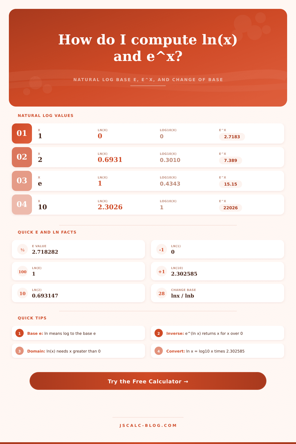
1	0.000000	0.000000	0.000000	2.718282
2	0.693147	0.301030	1.000000	7.389056
e ≈ 2.71828	1.000000	0.434294	1.442695	15.15426
3	1.098612	0.477121	1.584963	20.08554
5	1.609438	0.698970	2.321928	148.4132
10	2.302585	1.000000	3.321928	22026.47
100	4.605170	2.000000	6.643856	2.688×10^43
1000	6.907755	3.000000	9.965784	huge

📈e^x Exponential Table

x	e^x	ln of e^x	Note
0	1.000000	0	e^0 = 1 always
1	2.718282	1	e itself
2	7.389056	2	e squared
3	20.085537	3	e cubed
0.693147	2.000000	0.693147	ln(2), doubling point
2.302585	10.000000	2.302585	ln(10), a decade
–1	0.367879	–1	1 / e decay

🔗ln vs log10 Bridge

x	log10(x)	Factor	ln(x)
2	0.301030	× 2.302585	0.693147
5	0.698970	× 2.302585	1.609438
10	1.000000	× 2.302585	2.302585
50	1.698970	× 2.302585	3.912023
100	2.000000	× 2.302585	4.605170
1000	3.000000	× 2.302585	6.907755

≡Natural Log Identities

Identity	Rule	Example
Base value	ln(e) = 1	log of the base is 1
Unit value	ln(1) = 0	log of 1 is 0
Inverse	e^(ln x) = x	e^(ln 7) = 7
Inverse	ln(e^x) = x	ln(e^3) = 3
Power	ln(x^k) = k × ln(x)	ln(8) = 3 × ln(2)
Change base	log_b(x) = ln(x) / ln(b)	log2(8) = ln8 / ln2 = 3
ln to log10	ln(x) = log10(x) × 2.302585	ln(10) = 1 × 2.302585

⚙How The Base e Math Works

Natural logln(x) is the logarithm to the base e, where e ≈ 2.718281828. It answers: e raised to what power gives x?

Exponentiale^x is the inverse of ln. Feeding ln(x) back gives e^(ln x) = x, so the two operations undo each other.

Solve modeTo solve e^x = y, take the natural log of both sides: x = ln(y). This is why growth and decay problems use ln.

Change of baseAny log base b is built from natural logs: log_b(x) = ln(x) / ln(b). Set b = 10 for common log, b = 2 for binary log.

ln to log10Because ln(10) = 2.302585, you can convert: ln(x) = log10(x) × 2.302585, and log10(x) = ln(x) / 2.302585.

Domain checkln(x) is only defined for x > 0. ln(0) tends to negative infinity and ln of a negative number is undefined here.

💡Natural Log Tips

ln is base e: The "natural" log always uses base e ≈ 2.71828. When a formula writes ln without a subscript, the hidden base is e, not 10.

ln and e^x are inverses: They cancel out. ln(e^x) = x and e^(ln x) = x, so taking a natural log then an exponential returns your original value.

The mathematical constant is e. When mathematics deals with continuous change we use a special kind of number called the mathematical constant, e. Unlike integers which stay the same once they are given a value, e grow bit by bit. As such when dealing with continuously growing or decaying things the natural logarithm (ln(x)) is natural choice of function. Whether you’re modeling radioactive isotopes, bacterial cultures, or the growth of compound interest, e represent the rhythm of whatever is happening.

By and large, students remember that ln(e)=1 and ln(1)=0 but few understand where those numbers come from. The reasoning behind inputting certain numbers into a calculator are far more valuable than knowing how to spew out numbers on command. Calculators include ln and log buttons so what’s the need for a dedicated base? Calculus. One unique property of e is that its own derivative equal itself: (e^x)’ = e^x. No other number have that same property.

Why We Use the Number e

That makes e well suited for modeling continuous growth with minimal amount of math. Try cramming the equation into base ten instead and you’ll find yourself wrestling with ugly conversion factors all over the place. Economists and physicists love natural logs precisely because they strip away extra complexity from the problem. You can see the inverse relationship between e^x and ln(x) by toggling between them instantly on the calculator below. The former squishes huge ranges down to something more workable; the latter spread out tiny exponents into big numbers.

For example, think about the idea of doubling time from biology and finance. Given continuous growth over some period of time and a certain growth rate, how long will it take to double? To figure that out, divide ln(2)/rate. That’s because ln(2), roughly 0.693, gives us an easy way to eyeball how long something should of take to grow. No need to crank out differential equations for an approximation, just plug in the rate and voila! How long does it take to double? You’ll just need to use the drop down menu with popular rates already pre-filled.

And it doesn’t stop there; if you want to switch bases (perhaps you’re using log2 or log10 in your work) then you can do that too. It’ll show you both the natural log relationship as well as the translated version. That makes it clear that all logs is merely translations of each other.

One thing that people frequently forget about natural logs are their domain restriction. Ln(x) does not exist in the real number system as a function for zero or anything below that (negative). In fact, as you get closer and closer to zero from the right, ln(x) go off to negative infinity. That’s why you have a vertical asymptote at zero, which means on many theoretical models it would take an infinite amount of time to reach zero. And if you input something into the solver where e^x = y, what you’re actualy saying is “how long” is it going to take to achieve this target size? It’ll spit out one single number if it’s a positive y. Try putting negative targets and it will flag up an error. Continuous growth starting from positive can’t go back down through zero.

That’s why natural logs, ln(x), is frequently described as “the number you multiply x by to get log10(x)”. That number is indeed 2.302585, but it hides an intuitive understanding about the two bases: log10(x) counts orders of magnitude (each jump up from one integer to the next is multiplied by ten). In contrast, ln(x) measures compounded growth, specifically, its the continuous version of compounding, measuring the smooth curve that connects the discrete jumps of base ten. This distinction will guide your decision: If you’re comparing magnitudes (sound intensities, earthquake scales), use base ten; if you’re building a model of cooling rates or interest accruing, use base e.

The tables in the interface shows both simultaneously so you can visualize how they expand at different rates over the same input numbers. This stuff takes practice. It requires understanding the idea behind the number more than learning its value. This idea is based off continuous change: even though the number “e” stay the same, it describes something that is always changing. It’s the natural language of models for finance, wave mechanics, and probability distributions, as it explains the world at its grainy scale.

That “2.3” on your calculator screen after typing ln(10) isn’t just a number, it’s a window into that process of continual change. It measures how far you travel along a growth curve to get from one unit to ten times that amount. Though it might seem theoretical at first, once you put it to work, it make sense. Understand that all calculations represent continuous motion, motion that moves smoothly from instant to instant.