Z-Score Percentage Calculator
Turn any z-score into a percentage of the standard normal curve: area below, area above, area between two z-scores, or a two-tailed split. Optionally enter a raw value with a mean and standard deviation to find the z first.
📌Common Z-Score Presets
📝Z-Score Inputs
Primary z. In two-tailed mode the sign is ignored and ±z is used.
Only used when area type is between. Order does not matter.
Must be greater than 0. z = (x − µ) / σ.
🔢Formula Snapshot
📊Standard Normal Table (Cumulative %)
| Z-Score | Below Φ(z) | Above 1−Φ(z) | Between ±z | Two Tails |
|---|---|---|---|---|
| 0.00 | 50.00% | 50.00% | 0.00% | 100.00% |
| 0.50 | 69.15% | 30.85% | 38.29% | 61.71% |
| 1.00 | 84.13% | 15.87% | 68.27% | 31.73% |
| 1.28 | 89.97% | 10.03% | 79.95% | 20.05% |
| 1.645 | 95.00% | 5.00% | 90.00% | 10.00% |
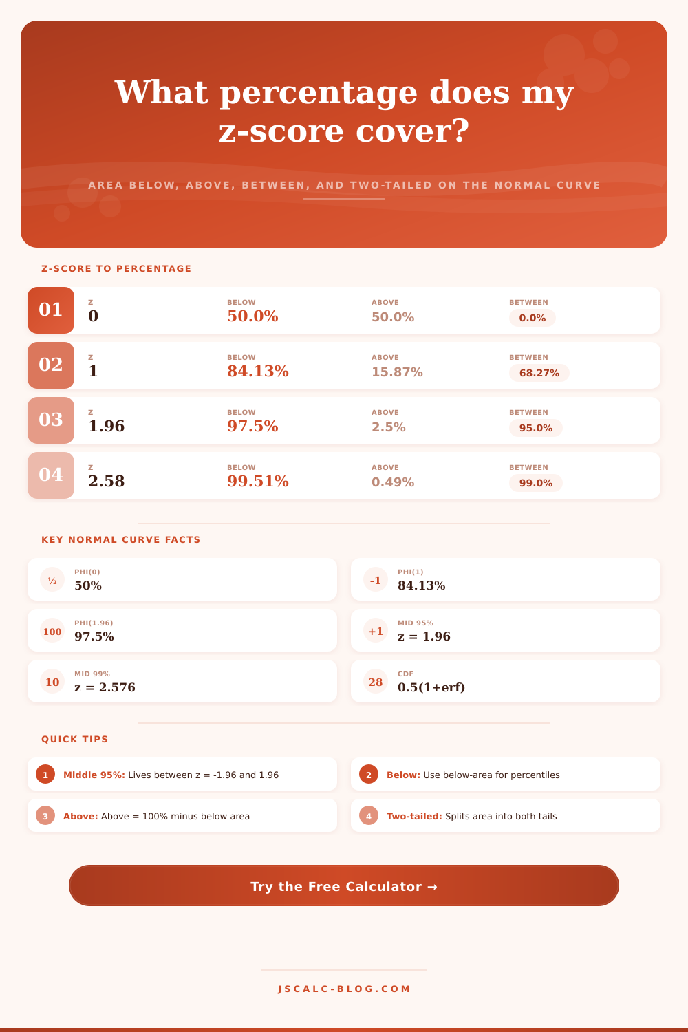
| 1.96 | 97.50% | 2.50% | 95.00% | 5.00% |
| 2.00 | 97.72% | 2.28% | 95.45% | 4.55% |
| 2.576 | 99.50% | 0.50% | 99.00% | 1.00% |
| 3.00 | 99.87% | 0.13% | 99.73% | 0.27% |
🎯Common Critical Z-Scores & Percentages
| Confidence / Use | Z-Score | Below | One Tail Above | Middle Between ±z |
|---|---|---|---|---|
| 80% confidence | 1.282 | 90.00% | 10.00% | 80.00% |
| 90% confidence | 1.645 | 95.00% | 5.00% | 90.00% |
| 95% confidence | 1.960 | 97.50% | 2.50% | 95.00% |
| 98% confidence | 2.326 | 99.00% | 1.00% | 98.00% |
| 99% confidence | 2.576 | 99.50% | 0.50% | 99.00% |
| 99.9% confidence | 3.291 | 99.95% | 0.05% | 99.90% |
📏Empirical Rule 68 / 95 / 99.7
| Range | Between ±z | Exact % | Each Tail | Both Tails |
|---|---|---|---|---|
| ±1 SD | −1 to 1 | 68.27% | 15.87% | 31.73% |
| ±2 SD | −2 to 2 | 95.45% | 2.28% | 4.55% |
| ±3 SD | −3 to 3 | 99.73% | 0.13% | 0.27% |
| Rounded rule | 1 / 2 / 3 SD | 68 / 95 / 99.7 | – | – |
⚖One-Tailed vs Two-Tailed Areas
| Z-Score | One Tail (above) | Two Tails (±z) | Middle Kept | Typical Alpha |
|---|---|---|---|---|
| 1.645 | 5.00% | 10.00% | 90.00% | 0.05 one-tail |
| 1.960 | 2.50% | 5.00% | 95.00% | 0.05 two-tail |
| 2.326 | 1.00% | 2.00% | 98.00% | 0.01 one-tail |
| 2.576 | 0.50% | 1.00% | 99.00% | 0.01 two-tail |
| 3.090 | 0.10% | 0.20% | 99.80% | 0.001 one-tail |
🗂Z vs Area Comparison Grid
| Z-Score | % Below | % Above | % Between ±z | % Outside ±z | Percentile |
|---|---|---|---|---|---|
| 0.25 | 59.87% | 40.13% | 19.74% | 80.26% | 59.9th |
| 0.50 | 69.15% | 30.85% | 38.29% | 61.71% | 69.1th |
| 0.84 | 79.95% | 20.05% | 59.90% | 40.10% | 80.0th |
| 1.00 | 84.13% | 15.87% | 68.27% | 31.73% | 84.1th |
| 1.50 | 93.32% | 6.68% | 86.64% | 13.36% | 93.3th |
| 1.96 | 97.50% | 2.50% | 95.00% | 5.00% | 97.5th |
| 2.33 | 99.01% | 0.99% | 98.02% | 1.98% | 99.0th |
| 2.58 | 99.51% | 0.49% | 99.02% | 0.98% | 99.5th |
⚙Full Formula Breakdown
📋Area Type Reference
| Area Type | Formula | Best For | Complement |
|---|---|---|---|
| Below (left) | Φ(z) × 100 | Percentile-style questions | Area above |
| Above (right) | (1 − Φ(z)) × 100 | Exceedance, upper tail | Area below |
| Between z1, z2 | Φ(z2) − Φ(z1) | Middle range coverage | Outside the range |
| Two-tailed | 2(1 − Φ(|z|)) | Two-sided significance | Middle kept |
💡Practical Z-Score Tips
Imagine you’re in class after taking a challenging statistics exam. Your friend got a 78 and you got an 82. Did she do better? That all depends on how difficult test was for both of you. Maybe the average score was 50, and there wasn’t that much variation between scores. In other words, your friend actualy did much better then you compared to the rest of class.
In a situation like this, z-scores can be helpful since they removes the raw scores from consideration and tell you exactly where you fall within distribution. The z-score represents how many standard deviations your value is away from mean. So it converts whatever normal distribution you have into one unified scale where you can compare different datasets.
Understanding Z-Scores and Percentiles
But sometimes, just knowing distance isn’t sufficient. Usually you’d like to know what percent of people is above and below you. That helps translate an abstract number into a concrete percentile. Now, instead of referencing some musty old textbook table of values, the above calculator does all of this math for you and translates those distances into accurate areas under curve. If you plug in your own z-score directly, it can calculates the area beneath it using the cumulative distribution function. That’s handy if you want to rank data since the area below any given value represent its percentile rank in sample exactly.
You’ll find that about 84 percent of population scored lower than you (meaning you performed at or above them) with a z of 1. The point at which most folks get hung up is on understanding what’s meant by one- vs. Two-tailed areas. In other words, you might want to know if something is just different in either direction than what came before it. To do that, you would calculate a two-tailed probability; the tool do this by double-counting the tail area outside your critical value. So when you look at, say, a Z-score of 1.96, that’s got 2.5 percent in each tail or 5 percent in total outside the mid-range. This explains why the default figure for hypothesis tests using 95 percent confidence intervals are 1.96.
You might be starting instead with some raw data that has not yet been calculated into a z-score. That’s fine, but the first important thing here is to get it into something called standardized form. To do so, you subtract the mean and then divide by standard deviation. This lets you compare different kinds of things in one statistical conversation, such as determining whether a particular rain storm was unusual compared to Phoenix or Seattle.
The calculator helps with this process: you can enter raw numbers (and the parameters that goes with them). For general guidance, the pages has reference tables you can consult to check common cutoffs. As you’ll see, roughly 68 percent of observations fall within one standard deviation and about 95 percent is included in two. While these can be helpful rule-of-thumb guidelines, if you’re doing real world analysis, you’ll need more precise estimates. For example, 99 percent of the center portion occur at a z-score of 2.576 with just 0.5 percent left on each end tail. That’s the kind of accuracy needed where financial or safety risk is at stake.
People usually get confused here by mixing up whether they are talking about being above or below mean. Under pressure it is really tempting to switch these in your mind. Take a moment and think; what side of the mean does my value fall on? If it’s positive then more of its area lies below, if it’s negative then more of its area lie above. This avoids confusing things because output clearly labels which region is being measured.
There’s more to statistical literacy than memorizing formulas: it’s also seeing that spread in your head. The calculations aren’t scary, they’re intuitive once you have an idea of where on the bell curve your number should of fall. You see this when grading tests, looking at defect rates in manufacturing, or reviewing results of medical tests. Knowing whether a number is higher or lower provide better insight than any single score alone. Numbers don’t lie…if you learn how to read the numbers’ context.