Variance of a Random Variable Calculator
Enter a probability table, percent table, raw sample, or frequency sample to calculate mean, expected square, variance, standard deviation, and row-by-row contributions.
Optional labels. Use one label per row; blank labels become Outcome 1, Outcome 2, and so on.
Enter one numeric x value per line, or separate values with commas, spaces, or tabs.
For probability mode, enter p(x) values. If they are close but not exact, the calculator normalizes them for contribution math.
Distribution audit table
| Outcome | x | Input weight | p(x) | x p(x) | x² p(x) |
|---|---|---|---|---|---|
| Results appear after calculation. | |||||
Variance contribution table
| Outcome | x - μ | (x - μ)² | Contribution | Share of variance |
|---|---|---|---|---|
| Results appear after calculation. | ||||
Which variance formula to use
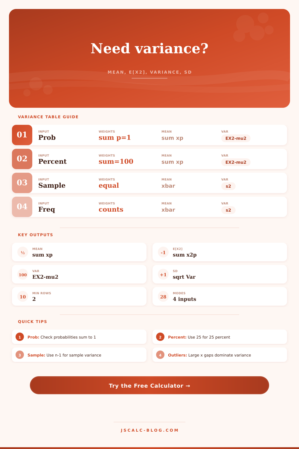
| Input type | Weights mean | Variance reported | Best use | Watch for |
|---|---|---|---|---|
| Probability p(x) | Given probabilities | E[X²] - μ² | Known discrete distribution | p values should sum to 1 |
| Percent probabilities | Percent divided by 100 | E[X²] - μ² | Forecast tables in percent form | Percent total should be 100 |
| Raw sample | Each row has weight 1/n | Sample s² with n - 1 | Observed data values | Need at least 2 rows |
| Frequency sample | Counts divided by n | Sample s² with n - 1 | Grouped observed counts | Counts must be nonnegative |
| Frequency population | Counts divided by N | Population variance | Complete finite population | Do not apply n - 1 |
Common random variable variance patterns
| Pattern | Typical x values | Shortcut variance | Table check | Interpretation |
|---|---|---|---|---|
| Bernoulli | 0, 1 | p(1 - p) | Two-row table | Spread is highest at p = 0.5 |
| Discrete uniform | 1 to k | (k² - 1) / 12 | Equal p(x) | Fair dice and equally likely ranks |
| Binomial count | 0 to n | np(1 - p) | Mass over counts | Repeated yes-no trials |
| Poisson count | 0, 1, 2, ... | lambda | Mean near variance | Event counts over fixed exposure |
| Two-loss risk | 0 and loss | p(1 - p) loss² | Two-row table | Rare large losses can dominate SD |
| Score frequency | Grouped scores | Use sample s² | Counts by score | Shows dispersion of observed group |
From that perspective, you’ll likely have some familiarity with variance, something you encountered in a stats course as a confusing obstacle to overcome. Sure, the equation was terrifying; and the example numbers was never particularly relevant. In practice, however, variance is nothing more than a way to calculate degree of surprise. How far off is actual result from what you thought?
Whether you’re evaluating risk, designing a product, or making a budget, understanding the mean isn’t even half of the story. You also want to understand just how crazy things could go. And that’s where this calculator gets interesting: It brings all of those listed ideas back down to Earth.
How Variance Helps You Predict the Future
First, know that not all data is created equal. Do you have a raw set of observations (e.g., your store’s weekly sales numbers) or do you have an entire distribution of probabilities (the chance of rolling each number on a six-sided die)? These are two entirely different types of inputs. Use the wrong kind of math and you’ll end up underestimating the variance.
To handle this, the tool allow you to define what sort of input you’re using. Both frequency samples and raw samples triggers the correct adjustment. This accounts for our lack of certainty when working with a small sample instead of an entire population. It is a tiny detail but one that helps avoid a very common analysis mistake.
Let’s compare a fair die to a loaded one for example. If we roll a fair die it will have even spread where each side is just as likely to occur. There’s little variation in the outcome. But what if we use a die that rolls a six nine out of ten times? The average changes a lot but the variation decrease (since the result isn’t so surprising). You can tell what’s going to happen. That’s the key idea with variance: the more certain something is the tighter its variance tends to be. The more uncertain the higher the variance.
Why does this matter? Because it allows you to determine if something is in control or headed toward chaos.
You’ll want to look at standard deviation, not the variance itself, when you look at the results. Variance is measured in units squared (which is mathematically convenient) but it’s confusing for humans. Twenty-five square dollars sounds like nothing if that’s your bank account. But a standard deviation of five dollars tells you something. It tells you what a typical amount differ from the average. So if your monthly expenses average $400 per month with a standard deviation of $50, then you’ve got a reasonably predictable budget. If your standard deviation were $300, then you’re flying blind. The calculator displays both, but the one you’ll actualy use to make decisions is the standard deviation.
Variance is disproportionately affected by outliers. Since it squares the difference between mean and observation, a single extreme observation has a greater impact than dozens of small-to-moderate observations. For instance, if you’re calculating variance of your insurance portfolio, a giant single loss will increase your variance far more then several smaller, moderate losses.
That’s why it’s so important to audit your data for errors. One typo, changing a “10” to a “100,” for instance, would of blown up your variance numbers. The tool shows you exactly what each row contributes, so you can spot which observations is pushing the variance. If one particular row is dominating the variance, then you want to know why before trusting the aggregate number.
In the end, this is all about setting; and resetting, expectations. It’s about capturing variance. Variance measures the noise from the signal. Variance applies whether measuring financial returns, manufacturing defects, or test scores: You want to reduce unnecessary variation around a desired mean. You want high average score. But you also want it to be consistent.
Let the calculator grind through the math; use that time to think about what the numbers tell you. Examine the spread, check the outliers, and know that a lower variance will typically result in a more predictable (and thus more easily managed) reality. That’s the true worth of the math, less the formulas, and more the ground.