Negative Binomial Calculator
Calculate exact, cumulative, and tail probabilities for the number of failures before r successes or the total trials needed to reach r successes.
🎯Scenario presets
📝Inputs
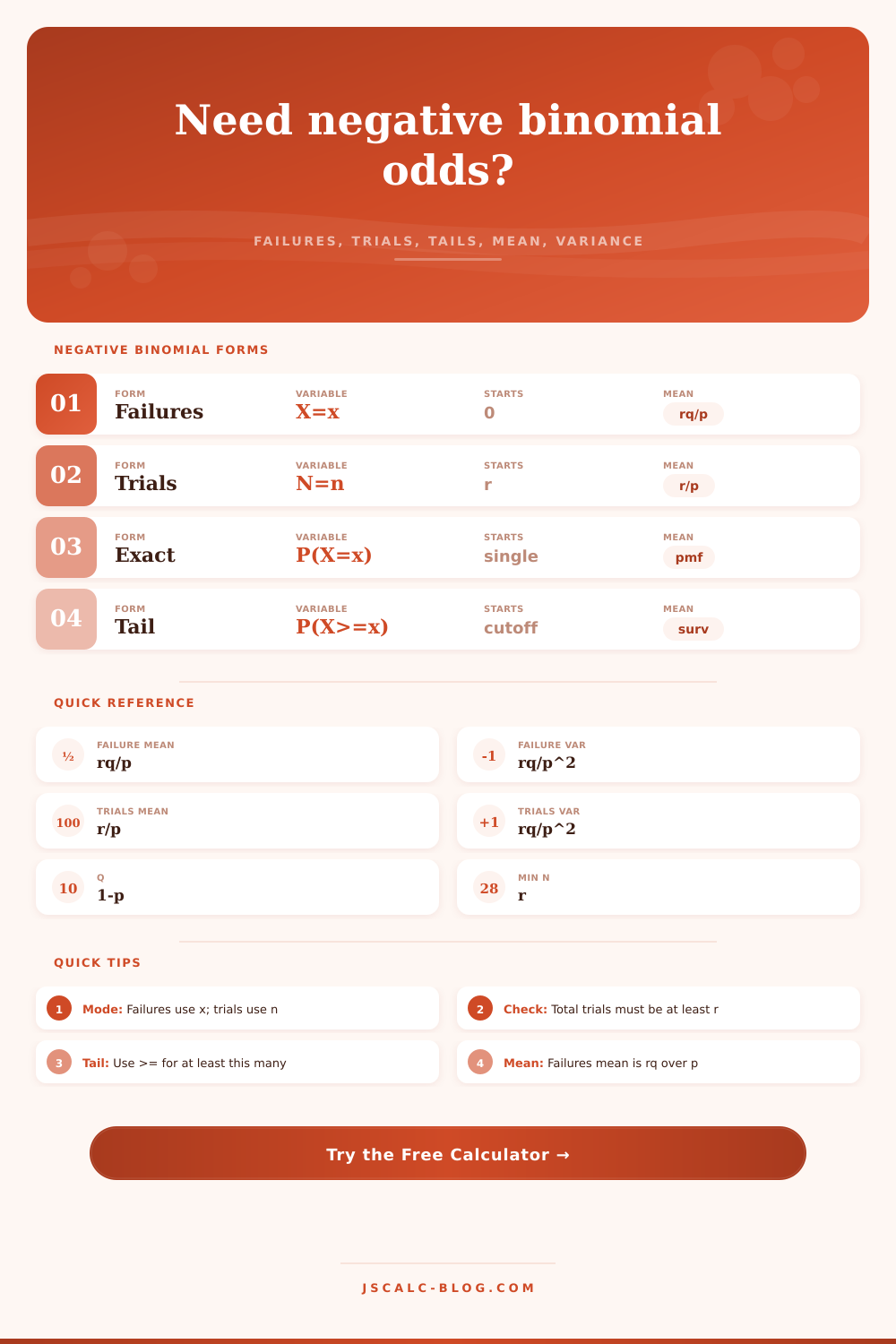
Failures mode uses X=x. Trials mode uses N=n and converts x=n-r.
Enter 40 for 40%, not 0.40.
The count of successes that stops the experiment.
Each independent trial has the same success chance p.
Used directly in P(X=x). In trials mode, x is synchronized from n-r.
Trials form uses P(N=n), where n must be at least r.
The result cards still show exact, cumulative, and survival values together.
Controls percent precision in result cards and generated tables.
🔢Current distribution snapshot
📊Distribution table around your input
⚖Preset comparison grid
📐Formula reference
| Quantity | Formula | Variable | Minimum | Use |
|---|---|---|---|---|
| Failures PMF | P(X=x)=C(x+r-1,x)p^r(1-p)^x | X | x=0 | Failures before target success |
| Trials PMF | P(N=n)=C(n-1,r-1)p^r(1-p)^(n-r) | N | n=r | Total trials to target success |
| Failure mean | E[X]=r(1-p)/p | X | 0 | Expected failures before stopping |
| Trials mean | E[N]=r/p | N | r | Expected total attempts |
| Failure variance | Var(X)=r(1-p)/p² | X | 0 | Spread in the failure count |
| Tail relation | P(X ≥ x)=1-P(X ≤ x-1) | X | x=0 | At least this many failures |
🧮Moment and cutoff table
⚙Method breakdown
💡Tips
JSCalc-Blog.com: This negative binomial calculator uses the standard failures and total-trials PMF formulas, cumulative sums, mean failures r(1-p)/p, and variance r(1-p)/p².
Let’s say you’re playing basketball and taking free throws. Until you have made five baskets, you’ll continue to shoot. How many shots do you think you’ll take? What matters isn’t the total number of shots you take, it’s how many times you miss while getting there. That’s what the negative binomial distribution describes. It describe the likelihood of seeing a certain number of failures before you reach a fixed number of successes.
So if you had an independent trial with a consistent chance of success, this would be a good model for predicting any situation that repeats itself until you hit a goal. Once you establish your chances of succeeding and the number of successes you want to see, the calculator does all the math. Then you can concentrate on what the results mean instead of getting bogged down in combinatorial math.
Understanding the Negative Binomial Distribution
So what’s the meat of this distribution? These are the parameters. We have two of them: p is the probability of a success on each individual trial, and r is the desired number of successes. (In most cases, the thing we’re interested in counting is x. The number of failures preceding our rth success.)
An alternate way of phrasing this is to ask how many total trials will be required, including the successes. This describes exactly the same situation as above but starting from slightly different points. In the case where we’re asking for the total trials, we start at r since it’s not possible to obtain r successes in less than r tries. On the other hand, in the case where we’re counting failures, we begin at zero, since there may be no failures at all! Depending on which form you choose to use, you’ll interpret your result different. Does it matter if you’ve planned for inventory or do you want to budget based off wasted material?
So what do the mean and variance tell us? The mean represents how many times you expect to fail. It’s r times q over p. So q is (one minus p). That means you’ll expect on average r/q failures. A high failure rate means you’re going to go through a lot of miss before you succeed.
How much variation should we expect? Variance has the same form, but is divided by p times p. So as your success probability decreases, the variance increases even faster. It means that while you may reasonably expect the above-average outcome, the real-world results could vary dramatically. Maybe you get lucky and hit your target right away. Or maybe you have a series of failures stretching out into the future.
The shape of the distribution is right-skewed. That means there’s a risk of long tails of bad luck. In practice, we tend to care less about precise probabilities as we do about tail probabilities. I mean, how much should it matter that there’s a 0.2% chance you get precisely three failures? That’s probably not actionable information. What matters is: what’s the chance I’ll have more than ten failures? What is the chance I’m going to blow through more than fifty sample?
It’s particularly useful for things like quality control. And the calculator gives those chances, survival and cumulative probabilities. You can see the chance that something exceeds some threshold. If you’re trying to predict sales, or perform quality control, this is huge. Say you need ten positive assay results; you don’t just want to know the chance of having exactly three failures, but you do want to know the chance that you will burn through more than fifty samples. The table on the page makes all this clear. It helps you plot where your inputs fall in the larger distribution.
Some common errors are mixing up the concepts of failure and trials. For example, it’s tempting to put the number of trials into an equation designed for failures. This makes a big difference in calculation even if the small details is missed. Another trap involves assuming independence. Trials has to be independent with the same chance of success for the negative binomial model to apply. That means that if you’re tinkering with something over time, whether developing skill at sports or breaking down machinery during manufacturing, then this model might not match your situation. It’s a snapshot model applied to a dynamic system; context counts. Make sure you understand whether your situation matches the assumptions before buying into the math.
This has practical applications when planning. The lessons apply equally to everyone. This includes a marketer trying to estimate call volume to get three sales, a researcher trying to understand how many samples are needed for a positive result, or a gamer who wants to know the drop rates for rare items. Set your goal, set your odds, and evaluate your chance of failure. The math makes the repeated trial and error easy to translate into a probability map. It lets you see average, the spread, and even the extreme risks all at once. It helps you assess risk and assign resources more effectivly. It removes guesswork and replaces it with knowledge about what’s statistically likely to happen.
The negative binomial distribution lets you handle your uncertainty when working through repetitive tasks. It recognizes that winning requires losing first. And it gives you a way to quantify how much losing costs you so that you can aim for the mean but plan for the worst case. It transforms an unpredictable series of wins and losses into a coherent system of chances. It provides a structure for understanding what’s probable, possible, and simply improbable. That knowledge will help you understand the odds in front of you and make informed decisions on where you should place your bets. Because when you do something repeatedly until it succeeds, there is no such thing as randomness, there is only data. And data always has a story to tell.