Geometric Distribution Calculator
Calculate exact, cumulative, and tail probabilities for the first success on trial k or for x failures before the first success.
🎯Scenario presets
📝Inputs
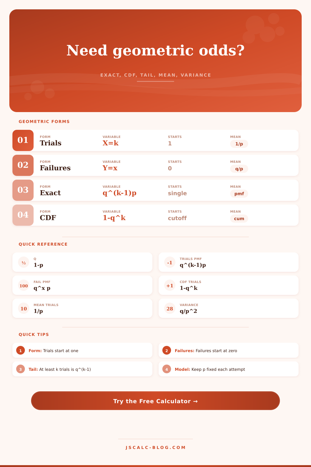
Trials start at 1. Failures start at 0 and equal k-1.
Enter 25 for 25%, not 0.25.
Each independent trial has the same success chance.
Use this for P(X=k), the first success on trial k.
Use this for P(Y=x). The synchronized trial count is k=x+1.
The result cards show exact, cumulative, and survival values together.
Used to find the trial or failure cutoff that reaches a chosen CDF.
Controls percent precision in cards and generated tables.
🔢Current distribution snapshot
📊Distribution table around your input
📋Preset comparison table
🧮Formulas and interpretations
🔍Common probability ranges
| Success p | Mean trials | Mean failures | 95% trial cutoff | Typical use |
|---|---|---|---|---|
| 1% | 100.00 | 99.00 | 299 | Rare drops, low response rates |
| 2% | 50.00 | 49.00 | 149 | Low-conversion outreach |
| 5% | 20.00 | 19.00 | 59 | A/B conversions, uncommon hits |
| 10% | 10.00 | 9.00 | 29 | Moderate response process |
| 25% | 4.00 | 3.00 | 11 | Skill attempts, support attempts |
| 50% | 2.00 | 1.00 | 5 | Coin-like independent trials |
| 75% | 1.33 | 0.33 | 3 | High-reliability attempts |
| 90% | 1.11 | 0.11 | 2 | Very likely first attempt success |
💡Tips
JSCalc-Blog.com: This geometric distribution calculator uses P(X=k)=(1-p)^(k-1)p, P(Y=x)=(1-p)^x p, CDF=1-(1-p)^k, and variance (1-p)/p².
The way we think about the anxiety of waiting for something special is all math. This includes things like getting your first yes from an employer who has rejected you multiple times, finally finding that legendary item in your favorite video game that has only a one percent drop chance, or being a quality engineer and having a part fall off conveyor belt and pass inspection. We’re waiting for the first “yes” in a series of independent trials.
That’s known as the geometric distribution, which tell you exactly the probability of getting our first “yes” on the k-th try … or earlier. After specifying the success rate, the calculator runs the numbers for you. You provide it with likelihood of success, usually expressed in decimal or percent form (i.e., 0.4 or 40%).
How to Use the Geometric Distribution Calculator
But first, you need to specify what type of problem you’re trying to solve. This is where many people mess up. There are two common ways to set up the geometric distribution problem, and choosing the wrong way will shift timeline by one step.
In the first formulation, you’re counting the number of trials required until the first success, including the trial where you do have a success. So if you get lucky on the very first try, then your count equals one. In the second formulation, you’re counting the number of failures before you finally achieve success. In other words, if you luck out on the very first go-round, your count is zero.
Why does the mean matter? Well, it tells you how much you should of expect to wait. For example, if the chance of success is 10%, then according to the mean, we’d expect to have to run through ten trials before finding our first success. But the distribution is heavy-tailed. This implies that even though the mean is ten, in practice, you may go ten, twenty, thirty, maybe even fifty trials without seeing a single success.
That’s where the variance comes into play. It measures the spread. A large variance is telling you that, in reality, your experience may be far off from what the average predicts. You’ll get lucky and do well right away or you’ll end up waiting quite a bit longer then average. The calculator gives you both so you can figure out not only where the middle of the distribution lies, but also how wide the distribution spreads out.
Finally, think about probabilities of tails. That’s the probability that you’ll wait past some threshold. This is typically the most important measure in business settings. For example, maybe your conversion rate for a marketing campaign is two percent. You’d like to know what the chance is that you’ll have to contact over one-hundred people before getting a single sale. The answer comes straight from the geometric distribution.
In fact, the geometric distribution is a survival function: it answers the question of the likelihood that you haven’t had the first success yet. Knowing that can help set expectations. It can also help you decide whether to pursue something or if it is worth spending time on it.
These are shown on the page with a reference table. You’ll see that the mean decreases rapidly with increasing probability of success. For example, if your success probability is one percent, then it takes one-hundred tries, on average. And if your success probability is 50 percent, it take two, on average. So the relationship between the two variables is not linear.
The mean wait time is halved when the success probability is doubled. That’s a very strong lever. When you operate something, getting the odds in your favor by just a bit has a huge effect on the mean wait time. That’s why improving success probabilities and conversion rates is a priority in ops.
Be mindful of what you’re asking. Are you looking at the probability of exactly three failures (failure mode)? Or are you interested in the probability of the first success being on the fourth trial (trials mode)? You’ll get the same numeric probability for this event from both approaches, however, they map to different integer values. The calculator offers the ability to change modes (which way the math works) based off how you phrase the question.
Additionally, it gives you cumulative probabilities (the probability that there has been a success by a specific point in time). That’s the inverse of a tail probability. Think about whether you’ll finish something by a particular date.
The assumption behind the geometric distribution is that each trial has nothing to do with last result. Your luck can change if you have some bad outcomes followed by good luck. But often you are operating within a more controlled environment, like a randomized experiment or a manufacturing line where this sort of independence is possible.
So while you’re never guaranteed to succeed, the geometric distribution give you a clean framework for thinking about how likely you are to succeed. This sort of clarity is helpful. It allows you to make a decision: should I keep trying? Or should I call it quits?
The randomness doesn’t go away. The math doesn’t take the randomness out of things, but it gives you a map. And a map is always better than wandering aimlessly.