Poisson Distribution Calculator
Calculate exact, cumulative, tail, and range probabilities for event counts when a steady average rate λ applies to a fixed interval.
🎯Deep scenario presets
📝Inputs
Used in the result wording and comparison tables.
Examples: arrivals, errors, defects, goals, claims.
Average count in one base period. Must be greater than 0.
Use 0.5 for half a period, 3 for three equal periods.
The exact PMF and CDF use this whole-number count.
For P(a ≤ X ≤ b). It is adjusted if above b.
Inclusive upper bound for the range probability card.
The result cards still show exact, CDF, range, and moments.
Used only for readable labels, not for changing the math.
Controls percentages and decimal probabilities in all outputs.
🔢Current distribution snapshot
🗂Use case comparison grid
Model calls, customers, tickets, or patients arriving in a fixed interval.
Estimate counts of defects per batch, board, roll, page, or inspection window.
Track alerts, outages, claims, or errors when the rate is steady enough.
Approximate goals or scoring events when counts are independent and sparse.
Use page or chapter averages to estimate exact and cumulative typo counts.
Compare crashes, arrivals, or incidents over equal time or distance units.
Summarize detector counts, colonies, photons, or signal hits by interval.
Approximate signups or responses when many independent opportunities exist.
📊Probability table around k
📍Cumulative cutoff table
🧮Preset comparison table
📐Poisson formula and method table
| Quantity | Standard formula | What it means | Current use |
|---|---|---|---|
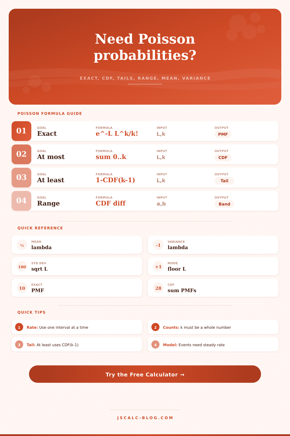
| PMF | P(X=k)=e-λλk/k! | Probability of exactly k events in the interval. | Exact probability card |
| CDF | P(X≤k)=sum from i=0 to k of e-λλi/i! | Cumulative probability through k. | CDF card and tails |
| Upper tail | P(X≥k)=1-P(X≤k-1) | Probability of k or more events. | At least selection |
| Range | P(a≤X≤b)=CDF(b)-CDF(a-1) | Probability inside inclusive bounds. | Range card |
| Mean | E[X]=λ | The long-run average event count. | Mean result |
| Variance | Var(X)=λ | Poisson variance equals its mean. | Variance result |
| Standard deviation | SD=sqrt(λ) | Typical count spread around the mean. | Snapshot grid |
💡Practical tips
JSCalc-Blog.com: This Poisson distribution calculator uses standard formulas for P(X=k)=e-λλk/k!, mean=λ, variance=λ, and CDF sums.
Right when you figure you’ve done enough for an hour, the phone rings. You look up at the clock, and you wonder whether it’s just bad luck … or is it simply a matter of statistics?
Enter the Poisson distribution, the home of that frustration. It doesn’t predict the future; rather, it helps you understand the beat of random systems that seem chaotic yet are regular. Plug in your average rate into the calculator above, and it’ll do the math for you. No need for you to guess at conversions and coefficients. Just see clearly what you can expect.
Understanding the Poisson Distribution
Lambda itself is the key parameter here: it’s the average number of events per fixed interval. So if your call center averages six calls per hour, then six is the anchor here. The tool will multiply that value by your interval multiplier, depending on which interval you are interested in, such as a half-hour shift. (So for example, for a half-hour shift, the effective lambda reduces from six down to three.)
This matters; probabilities behaves differently at different rates. When lambda is low, the distribution is shaped like a skewed-right thing with lots of probability on zero/one events and a long tail where there’s some tiny nonzero probability of really high counts. When lambda is high, it flattens out into something more bell-curve-like. The calculator does this part for you, but be aware that your choice of interval determines the game.
The interface will ask for some number k that’s the number you’re trying to observe. What are the chances of exactly eight calls? What about the chances of less than five calls? These numbers represent scenarios you can try running through the model.
If you work out the exact probability, it’ll tell you the likelihood of any one particular point. The cumulative distribution function adds up all the probabilities from zero up to that point. That’s the difference between them: it matters in planning. It’s academically interesting to know the exact probability of recieveing exactly eight calls. But what does that matter in operations? I need to know if my staff will hold up under the pressure. Is there a chance I’ll have at least as many calls as I can handle? That’s the part people get wrong. They pay attention to the spike, not the accumulation.
It can break down the range probabilities. This lets you ask, “What’s the chance I’ll have a count between five and ten?” I find that most helpful for deciding how to use resources. Instead of having one specific target, you get a buffer zone. On the page there’s a table of reference where they show you how the probability mass changes depending on what bounds you set. You can see that with a steady rate, extremely high or low numbers are exponentially unlikely.
The fact that the standard deviation is just the square root of lambda is a neat mathematical property. The standard deviation is simply the square root of lambda, which makes everything simpler. This ties the spread of your data directly to your average. As your average increases, your data becomes noisier but in a predictable way. For constant rate/independent events models, this is the sweet spot.
When there’s a spike in traffic from a viral post on your site, you no longer fit the steady-rate assumption. The underlying rate has changed too fast for Poisson to be useful for modeling the spike. A minor detail, but still: you need to believe that the past average is a good stand-in for what will happen next. If the rate is varying wildly over time, then just use simple historical percentiles, or maybe time-series analysis instead.
But when you’re dealing with something like manufacturing defects, hospital admissions, or server errors, the Poisson assumption checks out quite nicely. This is a model of rare-but-recurring events, which is exactly where it excels. A classic example is soccer goals. There is a preset for that. A goal is a rare, independent event, and the underlying skill level doesn’t vary from minute to minute in the game. So you can plug in numbers to find out how likely a high scoring affair is different than a shut-out. It converts some pretty abstract statistics into real expectations.
Another weird quirk here is that if you have a mean and a variance then that means you’re equally likely to get something around that number. In other words, that’s one way to tell whether the data really fits this distribution. You might have overdispersion (i.e., your variance is much bigger than your mean). Unfortunately, the calculator won’t check this for you, so again, you should of do a quick sanity check on your own data before taking the output at face value.
In short: Structure helps us tame uncertainty. It doesn’t remove randomness, but it packages it into a form where we can make better choices. If you’re hiring for a help desk or looking for typos on a manuscript, having some sense of what the probability curve looks like provides a strategic advantage. You no longer react to each blip, you expect them and react accordingly. The phone will ring again; this time, you’ll know the odds first.