Cumulative Poisson Calculator
Calculate Poisson lower-tail, upper-tail, exact, and range probabilities from a mean event count λ, then check mean, variance, and useful cutoffs.
🎯Scenario presets
📝Inputs
Direct mode uses λ as entered. Rate mode multiplies rate by exposure.
Poisson mean, variance, and expected count all equal λ.
Examples: calls per minute, defects per batch, tickets per hour.
Rate mode computes λ = rate x exposure.
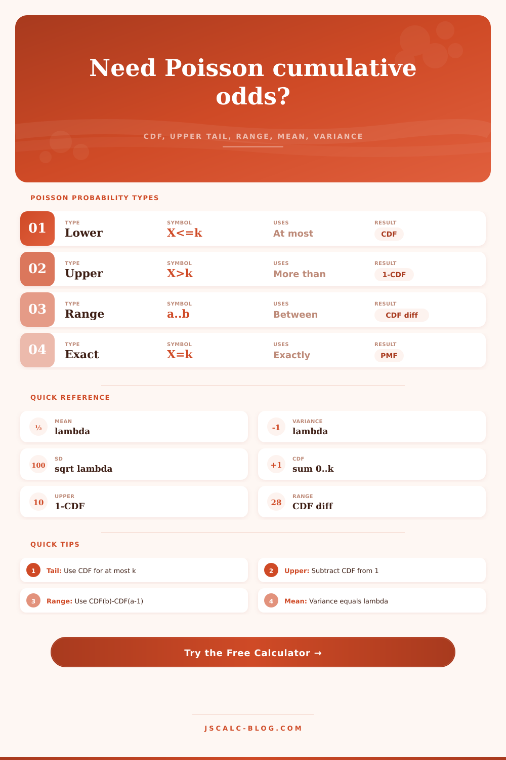
Lower tail is P(X ≤ k); upper tail is P(X > k).
Inclusive lower bound for P(a ≤ X ≤ b).
Inclusive upper bound. The calculator swaps a and b if needed.
Controls percent precision in cards and generated tables.
🔢Current distribution snapshot
📊Distribution table around k
🗂Preset comparison table
📐Probability method table
| Question wording | Probability | Formula | Includes k? | Calculator field |
|---|---|---|---|---|
| At most k events | P(X ≤ k) | sum from i=0 to k of e^-λλ^i / i! | Yes | Cutoff count k |
| More than k events | P(X > k) | 1 - CDF(k) | No | Upper-tail card |
| At least k events | P(X ≥ k) | 1 - CDF(k-1) | Yes | Distribution table |
| Exactly k events | P(X = k) | e^-λλ^k / k! | Yes | Exact card |
| Between a and b | P(a ≤ X ≤ b) | CDF(b) - CDF(a-1) | Both ends | Range inputs |
| No events | P(X = 0) | e^-λ | Only zero | Snapshot grid |
🔎Quick lookup table
🧮Formula notes
💡Tips
JSCalc-Blog.com: This cumulative Poisson calculator uses the standard Poisson PMF, CDF summation, upper tail 1 - CDF(k), range probability CDF(b) - CDF(a-1), and mean/variance λ.
Imagine you’re running a call center. On average, four calls per minute come through during your shift. The question haunting your shift is whether you will get more then six calls. The question is whether you will get more than six calls. These are rare, independent events that can be modeled using the Poisson distribution.
And you don’t have to be a mathematician to apply it. All you need to know is that random events take a predictable shape. Define your parameters and let the tool on this page do the rest. You will no longer need to do error-prone summations by hand.
How to Use the Poisson Distribution
Lambda (λ) is core of the model. Lambda is the average. Looking over a three hour period where you experience an average of 1.4 errors per hour, your lambda are 4.2. The calculator figures that out for you, but you need to make sure your units are correct. You’ll mix up your rates if you don’t. Your exposure might be in hours while your rate is per minute. That’s going to give you wrong answer. Double check your units before calculating. It is a small thing, but it matters.
Events is assumed to occur independently in the Poisson distribution. An error won’t cause another one. The model breaks down if they does.
Set lambda. Then select your cutoff. That’s k. It’s your definition of success or failure. It’s the number of events above which you’re in trouble. Below it you’re fine. (The cumulative distribution function tells you how likely you are to see k or fewer events.)
How does this help with capacity planning? Suppose you’ve got three agents and they can manages six calls. What are the odds that you’ll stay below six? The chance of staying below that number is provided by the calculator right there. It adds together all individual probabilities from zero up to k. A cumulative approach is helpful. Instead of a list of separate chances, you get one number that answers the question: That’s the risk metric.
The upper tail represent the probability of being over your threshold. That’s what’s left after you subtract the cumulative result from 1. If the upper tail probability is large, then you’re probably screwed.
In quality control, rather than just checking if something exceeds a number, maybe you’d like to see the likelihood that some number falls in a certain range. You can have the tool compute that as well (subtracting the cumulative probabilities of two values). It’s nicer than summing up all the little points. That is how they lay it out based off the table on the page.
There are multiple ways to say things. Each way has its own formula. Poisson: A poisson distribution has mean and variance equal to lambda. That’s neat for analytical purposes. You don’t have to worry about a parameter describing the mean and another one describing the spread. The square root of lambda is also standard deviation. So if you’ve got a low average count, there isn’t much spread. If you’ve got an average count of 1000, there will be more variance. High volume means there are wide swings in output for any given day. You can’t treat this as constant.
Mode: The mode is typically near lambda, a sort of measure of the middle value without having to perform any calculations.
But it takes patience to apply this to real problems. Reality breaks the independence assumption. Accidents is correlated with traffic; server errors are correlated with server crashes. When that happens, the Poisson model undercounts the likelihood of rare events. Inspect your data. Look for patterns. If the data clusters together, use a different distribution. But if the process is stable and random, Poisson works. It turns disorder into chances.
You know how much to budget for the improbable. How many people to staff for the probable. You’re left to read them in context. What do these probabilities tell you about your bottom line? Is it OK if you’re 10% likely to exceed capacity? That sounds fine. Fifty percent? That’s a crisis in the making. Adjust your resources to match. If the risk is too high, add more buffer. Add more buffer. Less than 50%? Maybe you’re overstaffed. You want to be right at the edge. Be prepared but not wasteful.
The tool helps you dial that number in. It turns abstract statistics into concrete decisions. The key: randomness isn’t noise. It’s a signal. The Poisson distribution describes the beat of random occurrences. It helps you anticipate the unpredictable … at least somewhat.
Can you ever know exactly how many will occur? No. But you can know the probability. And that makes all the difference. Instead of reacting to surprise, you’re planning against possibility. More than any specific calculation, this change in thinking matters. When you understand the form of randomness, you begin to see patterns where other people see disorder. That’s the true value of the Poisson distribution.