Hypergeometric Distribution Calculator
Calculate exact, cumulative, and tail probabilities when you sample without replacement from a finite population with a known number of successes.
🎯Scenario presets
📝Inputs
The math is the same; this label changes the interpretation text.
CDF values are computed by summing valid PMF terms.
Total number of items in the finite population.
Items in the population counted as successes or marked items.
Draws taken without replacement from the population.
The success count whose exact, CDF, or tail probability you need.
Controls probability percentages in the cards and tables.
Keeps the live distribution table focused near the observed k.
🔢Current distribution snapshot
📊Distribution table around your k
| k | P(X=k) | P(X≤k) | P(X≥k) | Band |
|---|---|---|---|---|
| Calculate to see nearby probability masses. | ||||
The highlighted row is your observed success count. Tail values are inclusive unless the selected statement says less than or more than.
🧮Formula and method reference
🗂Preset comparison table
| Scenario | N | K | n | k | Exact | Mean |
|---|---|---|---|---|---|---|
| Calculate to compare the built-in scenarios. | ||||||
📘Common hypergeometric situations
| Situation | Population N | Successes K | Sample n | Observed k | Best question |
|---|---|---|---|---|---|
| Card hands | Deck size | Target rank or suit | Cards dealt | Matches in hand | Exact or at least |
| Lot inspection | Lot units | Defective units | Audit pull | Defects found | At most or zero |
| Recall sampling | Shipped batch | Bad items | Checked items | Bad items seen | Detection chance |
| Tag recapture | Animals in area | Tagged animals | Recaptured set | Tagged recaptures | Exact count |
| Committee draw | Applicant pool | Priority group | Shortlist size | Priority selected | At least k |
| File audit | Total records | Flagged records | Review sample | Flags found | Tail risk |
| Survey subset | Respondents | Target answers | Manual review | Target answers seen | CDF check |
| Security logs | Log events | Suspicious events | Sampled logs | Suspicious hits | At least k |
💡Tips
JSCalc-Blog.com: This hypergeometric distribution calculator uses combinations, finite-population moments, and exact cumulative sums for sampling without replacement.
This problem isn’t one that calls for the binomial distribution. You’re pulling five cards and would like to calculate probability of getting exactly three hearts. Naturaly, most people will view every card as an independent event with a known (fixed) probability of 25% of being a heart. But that’s clearly incorrect; once you pull out a heart, it alter the makeup of rest of the deck, which in turn affects the probability of what you’ll pull next. This is precisely why we have the hypergeometric distribution: because the draws aren’t independent. This is math behind sampling without replacement. Whenever your population are finite and you can’t check off items and stick them back in pool, it comes into play.
The good news is, the calculator above does all of the combinatorics for you. There’s no need to work through the math to find combinations of thousands of thing. Instead, just set up the problem with following: First, enter overall population size. Next, enter the sample size. Finally, enter the number of successes from among those people. The tool will calculate exact odds of seeing exactly that many successes. It will also show cumulative results. Those can be even more helpful when making decisions, for instance, in quality control, you typically don’t really care about getting exactly two defects. You want to know the chance of getting two or fewer. That lets you know whether it’s probably an OK batch.
Why We Use the Hypergeometric Distribution
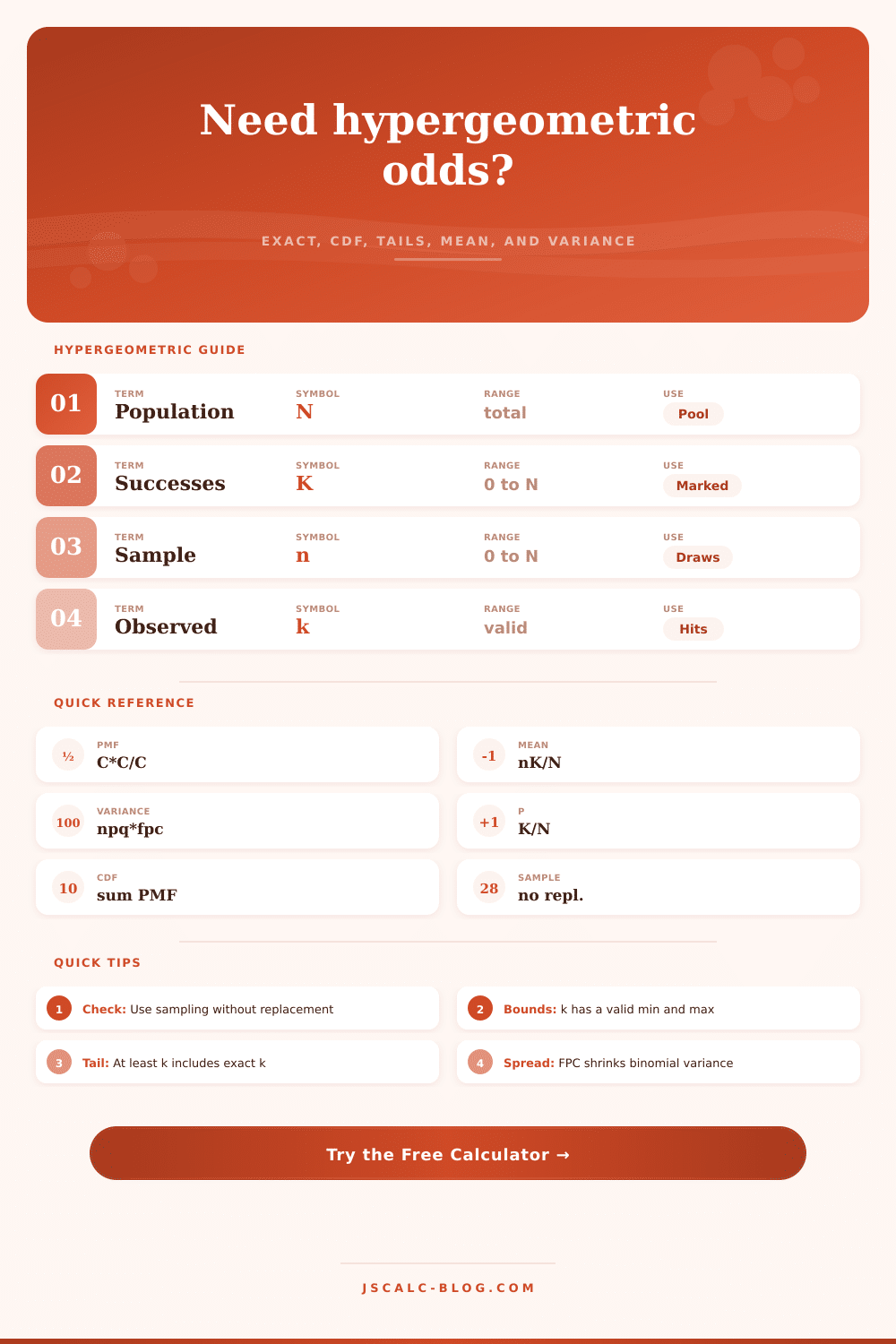
On the same page there’s a reference table that explains this nicely, it shows how each change moves you further down the distribution curve, and how the probabilities adjust accordingly. But then it’s all about understanding what we’re putting into it. Population size is how many things you are counting. Success Count is how many of those are successes (defective, got the right rank in a game, or are tagged with something). Sample size is how many things you look at. The Finite Population Correction Factor takes into account that if you take a large enough slice out of population, uncertainty decreases massively. You’ve covered so much of the population and seen such a large proportion of it that the numbers converges tightly on the mean.
Frequently these errors arise because people mix up boundaries with tails. For example: more than vs at least. More than begins at four; at least includes possibility that you get exactly three. The difference in probabilities is equal to probability of ending up at three. If three is close to the mode for this distribution, it could of make a big difference. The variance of the distribution also turns out to be very sensitive to what percentage of the population you include. When your sample size are small compared to the overall population it will behave nearly like independent trials. If you have a large sample but the population is small it will tend toward deterministic behavior.
And this distribution appears where you would least expect. For example, ecologists use this to measure animal populations through tagging/recapture experiments. You tag 100 animals and then recapture half of them. Based off the number of tagged animals that were recovered, the distribution can tell you something about the entire population. Financial auditors use this to evaluate risk in financial records. A few errors in a file? How likely are you to find those errors randomly with a sample? The hypergeometric model can help predict that. This is also an awesome way to test your own assumptions about detection and risk. And the tool’s built-in scenarios shows off its flexibility across many different areas, from jury selection to poker hands.
Finally, keep an eye on the range of outcomes that are actualy valid. You can’t pull out more successes than are present in population. You also can’t draw out more than there is items. The calculator adjusts for these bounds automatically. It doesn’t give you nonsense answers. It shows you what minimum/maximum number of successes could possibly be for your situation. This avoids the mistake of thinking the result is a symmetrical bell curve, sometimes it’s extremely skewed by extreme proportions or small numbers.
In the end, studying the hypergeometric distribution is to learn to appreciate the finite nature of our world. There aren’t infinite probability pools in life. Each decision alters the rules for following round. Understanding how these things depend on each other helps you make better decisions and estimate more accurately. Whether it’s an analysis of your survey response sample or the audit of a small batch of products, the math is identical. You’re working within a closed system, measuring the price of information. When you realize that each draw shrinks the pool of uncertainty, the equations stops being simple formula memorization. Instead, they become about following the movement of information. The deck does not forget what you have already seen.