Inverse Normal Distribution Calculator
Convert a left-tail, right-tail, or central normal probability into the matching standard z quantile and distribution-scale cutoff with x = μ + σz.
🎯Deep Scenario Presets
🧮Distribution Inputs
Central mode returns symmetric lower and upper cutoffs.
Use values strictly between 0 and 1, or between 0% and 100%.
0.975 decimal is the same as 97.5 percent.
Use 0 for the standard normal distribution.
Must be positive; x moves one sigma for each z unit.
Controls displayed z, x, density, and width values.
Examples: points, minutes, inches, percent, dollars.
📌Current Quantile Snapshot
area below x
input passed to inverse CDF
distance from the mean
single cutoff mode
left-tail area at upper cutoff
📐Formula Breakdown
🗺Probability Mode Reference
| Mode | What You Enter | Cumulative Area Used | z Result | x Result | Typical Use |
|---|---|---|---|---|---|
| Left-tail | Area below a cutoff | p | z = Phi inverse of p | x = μ + σz | Percentile, lower bound, pass mark |
| Right-tail | Area above a cutoff | 1 - p | z = Phi inverse of 1 - p | x = μ + σz | Top fraction, exceedance, alarm level |
| Central | Middle area between two bounds | (1 - p) / 2 and (1 + p) / 2 | two symmetric z values | lower and upper x values | Confidence bands and process ranges |
| Median | Left-tail 0.50 | 0.50 | 0 | μ | Center of any normal distribution |
| Lower tail | Small left probability | p near 0 | negative z | below the mean | Downside risk and low-percentile cutoffs |
| Upper tail | Small right probability | 1 - p near 1 | positive z | above the mean | High thresholds and screening limits |
📊Common z Quantiles
| Use Case | Left Area | Right Area | Central Area | z Cutoff | Two-Sided Bounds |
|---|---|---|---|---|---|
| Median | 0.5000 | 0.5000 | 0.0000 | 0.000 | center only |
| One-sided 90% | 0.9000 | 0.1000 | 0.8000 | 1.282 | -1.282 to 1.282 |
| One-sided 95% | 0.9500 | 0.0500 | 0.9000 | 1.645 | -1.645 to 1.645 |
| Central 95% | 0.9750 | 0.0250 | 0.9500 | 1.960 | -1.960 to 1.960 |
| One-sided 99% | 0.9900 | 0.0100 | 0.9800 | 2.326 | -2.326 to 2.326 |
| Central 99% | 0.9950 | 0.0050 | 0.9900 | 2.576 | -2.576 to 2.576 |
| Three sigma band | 0.99865 | 0.00135 | 0.99730 | 3.000 | -3.000 to 3.000 |
| Very high screen | 0.9990 | 0.0010 | 0.9980 | 3.090 | -3.090 to 3.090 |
🧪Preset Scenario Comparison
| Preset | Mode | Probability | Mean | Std. Dev. | Approx z | Approx x | Interpretation |
|---|---|---|---|---|---|---|---|
| IQ 98th Percentile | Left | 0.98 | 100 | 15 | 2.054 | 130.8 | Score at the 98th percentile |
| Exam Top 10% | Right | 0.10 | 72 | 9 | 1.282 | 83.5 | Cutoff for highest tenth |
| Central 95% Spec | Central | 0.95 | 50 | 4 | +/-1.960 | 42.2 to 57.8 | Middle specification band |
| 99.73% Process Band | Central | 0.9973 | 24 | 0.08 | +/-3.000 | 23.76 to 24.24 | Three-sigma process range |
| Slowest 2% Delivery | Right | 0.02 | 36 | 7 | 2.054 | 50.4 | Time exceeded by 2 percent |
| 1% Downside Return | Left | 0.01 | 8 | 12 | -2.326 | -19.9 | Lower one-percent outcome |
| Central 80% Forecast | Central | 0.80 | 1200 | 180 | +/-1.282 | 969 to 1431 | Middle forecast interval |
| Adult Height 90th | Left | 0.90 | 67 | 3.5 | 1.282 | 71.5 | 90th percentile height |
| Sensor Alarm 0.5% | Right | 0.005 | 0 | 1 | 2.576 | 2.576 | Upper anomaly threshold |
| Central 90% Calls | Central | 0.90 | 220 | 35 | +/-1.645 | 162.4 to 277.6 | Expected daily call band |
⚙Method and Accuracy Notes
| Step | Calculation | Why It Matters | Common Mistake | Calculator Handling |
|---|---|---|---|---|
| Validate p | 0 < p < 1 | Normal quantiles are infinite at exactly 0 or 1. | Entering 100% for a finite cutoff | Warns before calculating |
| Convert units | percent / 100 | Percent and decimal inputs must land on the same probability scale. | Typing 95 while decimal mode is selected | Separate unit selector |
| Invert CDF | z = Phi inverse of p | This finds the standard-normal cutoff before scaling. | Using a z table in the wrong tail | Acklam rational approximation |
| Scale result | x = μ + σz | Any normal distribution is a shifted and stretched standard normal. | Adding variance instead of standard deviation | Uses sigma directly |
| Central area | tail = (1 - c) / 2 | The outside probability is split equally across two tails. | Putting all leftover area in one tail | Returns lower and upper bounds |
| Report tail | 1 - p or split tails | Tail area explains how rare the cutoff is. | Calling a right-tail area a percentile | Shows cumulative and tail values |
💡Practical Quantile Tips
Consider a standardized test, for instance. You’re familiar with typical test scores, you know the mean and you know the range of test scores among people. You’d like to know the cut off between the top 10% of scorers and everyone else.
This isn’t a question of finding the probability based off their score. Rather, this is the opposite. You have the percentage in your hand and you seek the number which defines it. An inverse normal distribution calculator turns the typical bell curve maths upside down.
What Is an Inverse Normal Distribution Calculator?
Most of us will be taught to find the area underneath the curve. The other way around (i.e., seeking the point on the axis corresponding to the area) is a different matter entirely. It involves reversing the cumulative distribution function. For this the calculator above do all the hard work so you don’t have to get tangled up in complicated lookup tables or algorithms.
Once you understand how the scaling works, the guts of the thing are pretty straightforward. First, it applies to the familiar standard normal distribution. You know, the bell curve where the center point is zero and the width is one.
Next, it finds the z score for your desired probability. Z is simply the number of standard deviations you fall above (or below) the average. Positive z means above, negative z means below. Then, finally, it scales and moves this standard answer to fit your specific problem.
The equation is x = mu + sigma * z. Mu is your mean, sigma is your standard deviation, and z is the z value for which you want an answer. This is where the magic happens because in real life, the numbers generally won’t line up with the standard setup. Factory parts don’t weigh the same as humans do. They also differ in variation. Same goes for test scores. The calculator make these adjustments for you.
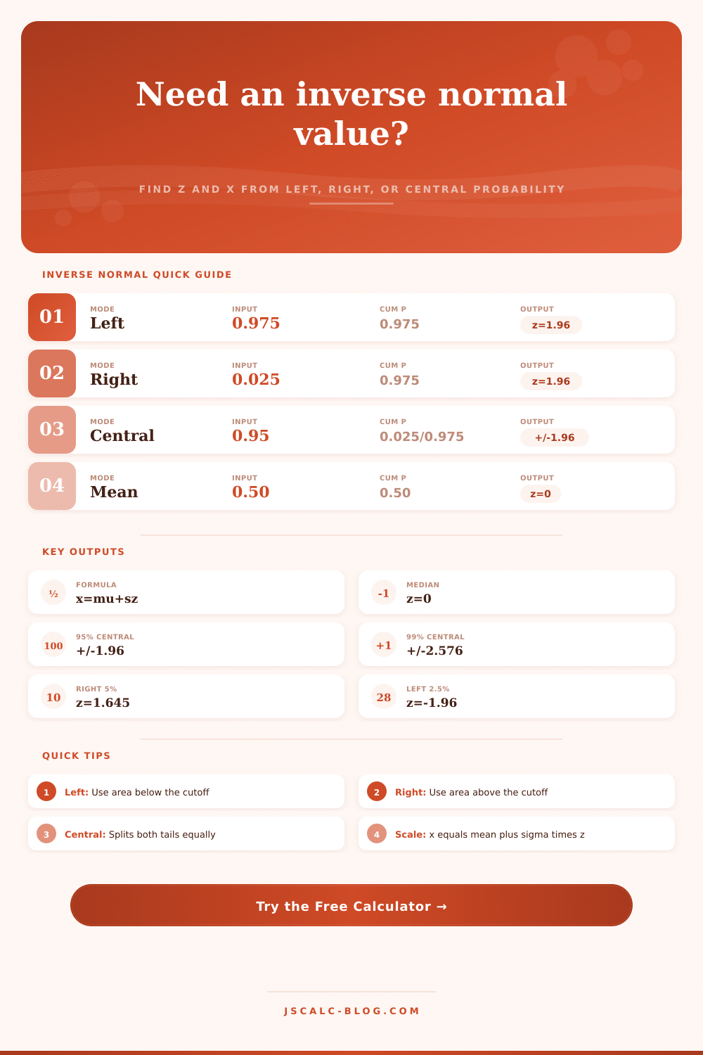
As you can see, there are three modes for entering your probability. There are three modes. The left tail is the easiest. Enter the area on the left of your cutoff and it returns the X.
Right tail is handy if you’re interested in exceedances. Perhaps you’d like to know how much rain fell that was exceeded only one percent of the time. Use that tiny tail end to find the extreme threshold.
Central mode is for intervals. It divides the leftover probability evenly between the two tails. This is what creates confidence bands. Enter the chunk in the middle that you’d like captured and it’ll return the upper and lower bounds. That symmetry are important for predicting and quality control.
Most mistakes occur here, when choosing which mode to use. It’s easy to confuse a right tail area with a left tail percentile. A right tail of 0.05 is the same cutoff as a left tail of 0.95. But the stories are different. The one is the bottom ninety five. The other is the top five.
Guessing what the user wants doesn’t make sense for the calculator. So it makes you pick which one it is, that forces you to think clearly about it. And it also protects against an all too common error: using the distribution twice for two sided tests. In the main mode, the tool splits the tails for you. And balances them.
The normal distribution is a model, not a law of physics. In the real world, things get messy. Many natural phenomena fits the normal distribution very well, but the tails of the distribution fail when extreme events occur. Natural disasters and financial crashes tend to have fatter tails then the normal distribution suggests.
The inverse calculator assumes that the distribution is normal and provides you with exact numbers. These numbers assume normality and are only as good as that assumption. If your data has skew, then the z scores will mislead you. First check your data. Look at the histogram. If it looks like a bell the tool is your friend. If it looks like a hill or a cliff, then you need a different approach. The math is sound but the model might not be.
It is a single number. It is definitive and comforting. Keep in mind, however, that it’s an estimate. Your sigma could very well be incorrect if your sample size was small. And guess what? That propagation error feeds right back into your cutoff. A little bit of inaccuracy with the spread equals a lot of inaccuracy with the threshold.
This is reflected in the calculator above. Tweak the standard deviation just a little and notice how it changes the cutoff. It reminds you: precise inputs result in precise outputs. Garbage in garbage out.
It is a translation. It translates abstract probability into concrete boundaries. Translation from a percentage to a price, to a score, to a measurement. And that translation is powerful. Because it lets you apply risk tolerance. It lets you make decisions and set limits. Scholarship cutoffs or alarm levels on a sensor? Same logic. Define the risk, find the boundary, and act to match it.
And that’s where the bell curve comes in. It provides the map. This calculator helps you plot your place on it. You begin with a percentage and you end with a decision. And that’s the value of inverting the problem.