Exponential Distribution Calculator
Compute waiting-time PDF, CDF, survival probability, mean, variance, standard deviation, interval probability, hazard rate, and percentile from one rate parameter.
Used for labels only; the math is the same exponential model.
Events per selected time unit. Must be greater than zero.
Keep x, a, and b in this same unit.
The waiting time where PDF, CDF, and survival are evaluated.
Enter as a probability from 0 to 1, such as 0.95.
Lower bound for P(a < X < b).
Upper bound for P(a < X < b). It should be greater than a.
Controls displayed probabilities and time values.
Calculation Breakdown
| Time point | PDF f(t) | CDF P(X <= t) | Survival P(X > t) | Meaning |
|---|---|---|---|---|
| Run the calculator to fill the probability table. | ||||
| Percentile | p | Time xp | CDF check | Survival left |
|---|---|---|---|---|
| Run the calculator to fill the percentile table. | ||||
| Question | Expression | Formula used | Result | Interpretation |
|---|---|---|---|---|
| Run the calculator to fill interval and tail checks. | ||||
| Use case | Typical rate meaning | Best question | Watch for | Model note |
|---|---|---|---|---|
| Queue arrivals | Arrivals per minute | Wait until next event | Rush-hour rate shifts | Works best with steady random arrivals |
| Reliability | Failures per hour | Survive past time x | Aging or wear-out parts | Constant hazard is assumed |
| Service time | Completions per minute | Finish by deadline x | Multi-stage jobs | Single memoryless stage is implied |
| Network gaps | Packets per second | Gap longer than x | Bursty traffic | Use short steady windows |
| Alert events | Alerts per day | Long quiet period odds | Scheduled scans | Independent event timing is assumed |
| Decay timing | Events per unit | Time to next count | Detector dead time | Rate should match observed conditions |
But time seems to pass slower then it actualy does. Three minutes on a clock feel like an eternity while sitting at a counter. That’s not how your brain calculates delay, it distorts time. And that’s what exponential distribution models: the amount of time until next event in a random series of events. When asked “when will the next thing happen?”, if process is memoryless, then it’s described by exponential distribution.
Plug in the probabilities and let the calculator do the math for you, translating ideas back into real estimates of time. Rate is the key part of model: we call it lambda (λ). Lambda equal event frequency per time unit. For example, if you have a server that receives twenty-five requests an hour then λ = 0.25 requests/hour.
Understanding Exponential Distribution
Note that the time unit for your rate should be consistent with unit used for your time variable. This is where folks get tripped up the most: they use a mix of units like minutes and hours without converting. That immediately destroys the calculation. The tool prevents this from happening because it allows you to set your desired time unit at the top of page. This way, all density and cumulative values show what you are trying to achieve.
The key feature of the exponential distribution, which distinguishes it from other distributions, is that it’s memoryless: The time you’ve spent waiting so far doesn’t affect your chances of getting hit by next event within the coming minute. A machine with a 10-hour uptime has no better or worse chance of failing during upcoming hour than when it began.
It turns out this odd quality holds true for radioactive decay and random arrival times, but not deterioration of aging components like car parts. And that is why model doesn’t work for wear-out components. It creates dangerous overconfidence about how long systems will last.
It also spits out several values, each appropriate for various types of decisions. The probability density function (which is useful for theoretical checks) reflect the probability of something occurring at any particular moment in time. The cumulative distribution function indicates the probability that wait is below some amount. That’s frequently more realistic for service level agreement purposes. Want to know the probability that a customer will be served within five minutes? Consult the cumulative value at five.
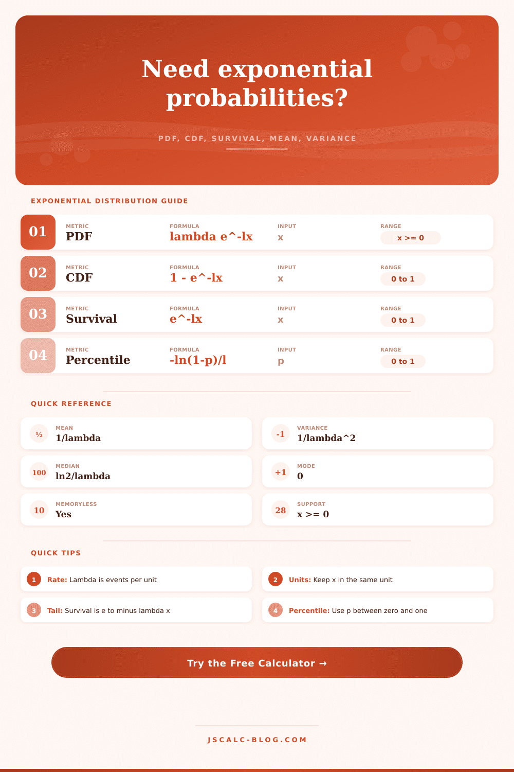
The survival function is the complement, indicating the probability the wait would be longer than that. There are also important metrics like mean and variance. Mean just refers to the rate’s reciprocal, or the inverse of it. So if your rate is 0.25 events/hour, your mean (or average) wait time are four hours.
Variance is equal to the mean squared, which tells you how widely distributed waiting times are. High variance implies that some people will get really long waits while others get super-short ones. And this is where queue frustration arises. Even with a reasonable average wait time, the distribution ensure that some individuals experience extreme delays.
You can understand percentiles by how they are used to manage resources and expectations. Because the distribution has a long right tail, the mean wait time will tend to be longer than median (often). The small set of extremely long waits will drag it upwards. The 90th percentile is the time point at which 90% of all events are completed. That sounds like an important number for setting realistic deadlines and allocating buffer times. It is good that it is also calculated automatically, so you would of not need to fiddle with logarithmic formulas yourself.
You can consider risk within a certain time frame using probability tables. For example, what’s the likelihood of something happening at 1-6 hours from now? That could be handy when planning to staff a shift or schedule maintenance. Here’s the table on their site that breaks it down nicely (how likely events are to happen over time). That will help you see where most of the action is.
From the delay of packets on a network to waiting in line at customer service, these are all real world examples that can be modeled using exponential distribution where we assume a constant hazard rate. This assumes a constant hazard rate, which means the probability of an event occurring in the next minute does not depend on how long you have already waited.
The simple exponential model won’t work if your arrivals vary over time (e.g. The number of customers arriving varies based off time of day). Here you might have to split up your data by time of day or model it in more complex ways. But if we’re dealing with a process in a state of balance then the simple exponential distribution is a powerful tool. It takes uncertainty and makes it manageable through numbers.
To conclude. Waiting time equations ultimately come down to setting your expectations. Does waiting seem like a long time? That doesn’t change no matter what the math says. But it also helps you estimate how much longer it’s going to be. These same principles apply whether you’re designing a system, or just frustrated by being put on hold. Patterns emerge from randomness, and knowing the pattern puts you ahead of the game. You can still wait forever, but at least now you know the odds.