Uniform Distribution Calculator
Calculate continuous uniform PDF, CDF, interval probability, mean, variance, standard deviation, and percentiles, with an optional discrete integer mode.
🎯Scenario presets
📝Inputs
Continuous uses density. Discrete uses equal probability mass.
The left endpoint of the support. In discrete mode it is rounded.
Must be greater than a for continuous mode.
PDF or PMF and CDF are evaluated at this value.
Lower value for P(L <= X <= U), clamped to the support.
Upper value for interval probability.
Enter p from 0 to 1, such as 0.25, 0.5, or 0.95.
Controls card values, percentages, and generated tables.
🔢Current distribution snapshot
📊Probability table around your value
| x value | PDF or PMF | CDF P(X<=x) | Right tail | Position |
|---|---|---|---|---|
| Calculate to fill the probability table. | ||||
📋Preset comparison table
| Scenario | Type | Bounds | x | CDF | Mean | Variance |
|---|---|---|---|---|---|---|
| Calculate to compare the built-in scenarios. | ||||||
📈Percentile lookup table
| Percentile | p | Continuous value | Discrete value | CDF check |
|---|---|---|---|---|
| Calculate to fill percentile cutoffs. | ||||
📘When a uniform model fits
| Use case | Uniform variable | Bounds mean | Good question | Watch for |
|---|---|---|---|---|
| Arrival window | Time inside stated slot | Earliest and latest time | Chance before a cutoff | Peaked traffic patterns |
| Manufacturing | Error within tolerance | Low and high tolerance | Chance inside spec band | Centered normal errors |
| Simulation | Random draw between 0 and 1 | Generator minimum and maximum | Percentile or threshold | Integer rounding choices |
| Audits | Random item number | First and last eligible item | Probability of an item range | Sampling without replacement |
| Scheduling | Jitter or delay amount | Smallest and largest delay | Tail after a limit | Clustered delays |
| Games | Fair spinner or die face | Lowest and highest face | Mass at one outcome | Unequal face weights |
🧮Formula and method reference
💡Tips
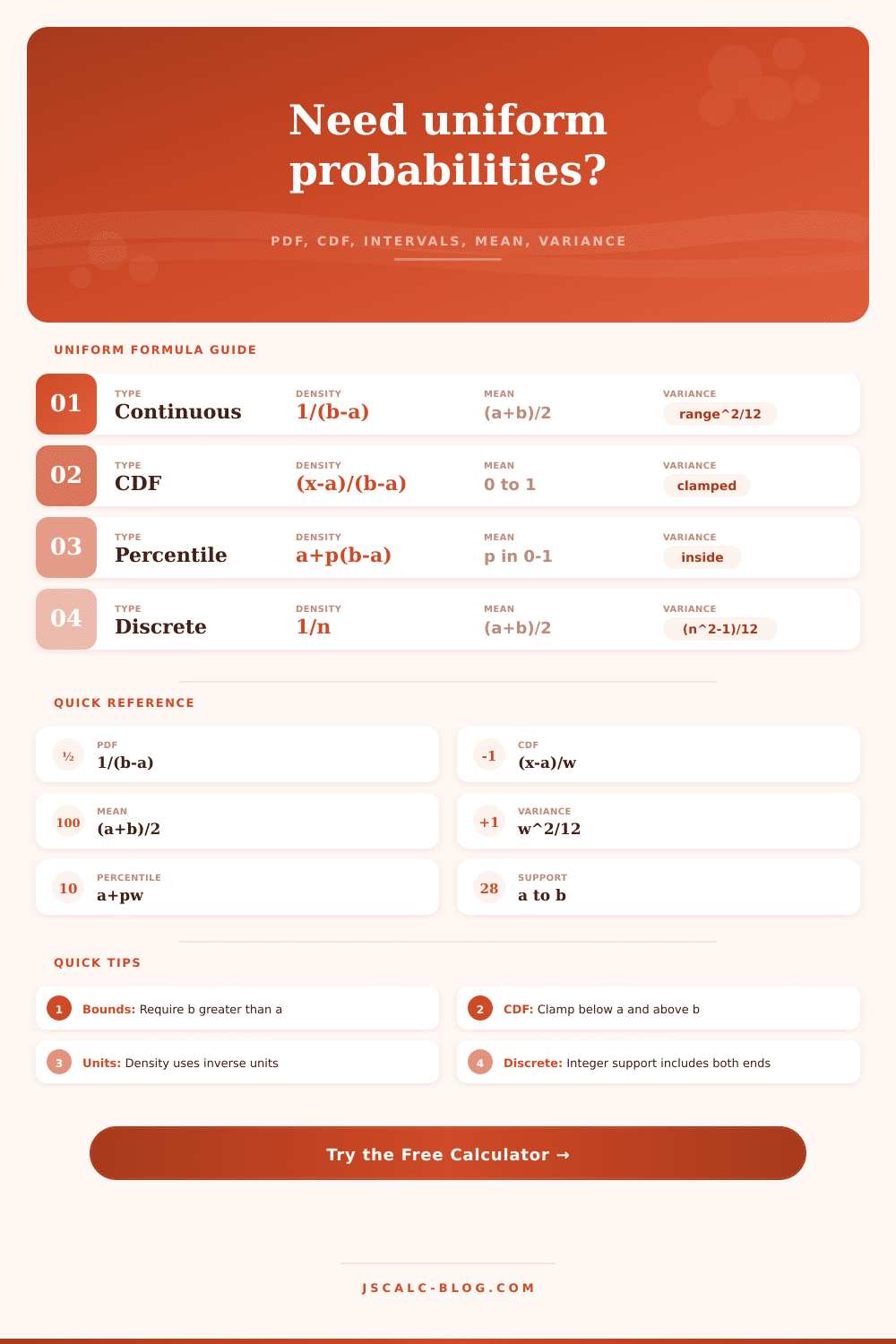
JSCalc-Blog.com: This uniform distribution calculator uses PDF=1/(b-a), CDF=(x-a)/(b-a), mean=(a+b)/2, variance=(b-a)2/12, and percentile=a+p(b-a) for continuous models.
If you think about randomness, chances are you imagine chaos. It is a disorderly mix of everything happening everywhere at once, a mess. But hidden within that chaos is a certain sort of order and it turns out to be quite flat. The math behind situations in which each possible outcome has an equal chance is known as the uniform distribution. In probability theory, it’s the example of pure fairness. It’s what you invoke when picking a number at random or spinning a fair dial.
Understanding it will change the way you think about timing and risk in your life. It’s straightforward: you specify an upper bound, a lower bound, and everything in-between happens equally often. There’s no bias toward one value versus another. That seems so simple, but that’s what makes it deceptive. In reality, life isn’t flat. Some traffic gets jammed together; people like certain numbers; errors clump around the average.
What Is Uniform Distribution?
Wherever there’s deliberate randomness or ignorance, the uniform model works. You have no idea when a bus will arrive, except that it will be sometime between 10 and 20 minutes. In this case, the uniform distribution is as good a place to start as anywhere. It models maximum uncertainty bounded by known values.
What’s the difference? Is this a continuous variable, where anything in the range is allowed like temperature or time? Or is it a discrete variable that jumps to the next whole number such as inventory counts or a die roll? Our calculator works in either mode without requiring any input from you to account for diffrent than the other. For example, instead of having two different equations to learn, one for discrete and another for continuous; we tweak the math to cover both bases. This happens under-the-hood: the probability mass function give each integer point an equal weight; whereas the density function remains constant throughout the interval. It may seem minor, but it makes all the difference in correctly computing exact probabilities. Get it wrong and you’ll be out by a multiple of the interval size.
Given those bounds, the tool then calculates something called the cumulative distribution function, or CDF. That’s the probability that some value is less than some other value. If I want to know the probability my delivery will arrive by one thirty when I have a delivery window between noon and two PM, I can use the CDF to figure out the answer. It doesn’t require any integration of a curve. Because the CDF of a uniform distribution is just a straight line, it’s easy to calculate. As you go up in value from the lower bound to the upper bound, the probability keep increasing. It starts at zero and ends at one.
The usefulness of the uniform distribution comes from its linearity. There’s two other critical outputs: mean and variance. The mean is just the midpoint of the interval. That’s the balance point in the distribution. But then there’s variance… Which tell us about spread. More variance = more unpredictability (i.e., wider interval). From here we get the standard deviation, which tells us by how much values tend to differ from the mean.
When you have a narrow distribution, the mean can be a good predictor. When it is wide, it doesn’t help at all because outcomes are spread out around the mean. It’s an intuitive tradeoff that people miss a lot, they fixate on the average, but not how scattered the actual data is.
In practice, this means the model is most powerful when applied to interval probabilities. Rather than requesting the probability of seeing a specific value (which will typically be zero in a continuous case), it requests the probability of observing a range of values. That’s what people do. We care about windows of time, ranges of prices, or bands of acceptable error. We’re interested in ranges, not specific values.
The tool makes sure that the probability input doesn’t go negative or above 1.0. It takes care of edge cases for you. Simply make sure your bounds make sense for the problem. So, don’t make your data fit the uniform model if it obviously clusters. If the observations bunch up in the center, then you want a normal distribution. If they cluster on one side, then try something like gamma or exponential.
The uniform distribution has its place. It can be used as a model for something random (like delays), as the distribution for input variables for simulations, and as a way of modeling things where you have no prior information about what values are more likely. But it’s a lousy model for physical processes with natural centers and human preferences. It’s fine for those jobs only if flatness is an assumption, not reality.
Here, it’s less important what the calculator gives you than how well you judge whether the model fits. But in short, what the uniform distribution does for you is it makes you appreciate the range. That’s the universe of possibility, and everything outside the range is just noise inside of those boundaries. Calculating the percentiles and probability correctly helps you transform that noise into useful insight.
Stop guessing, start measuring. A flat line isn’t boring; it’s honest. Honesty is a strong measure in a world where most data is skewed.
Wait, I realized I should of checked the math again before writing this. The uniform distribution can absorbs many different types of error. Actualy, when you are looking at furnitures, you see these patterns too. It could be more luxurius to use something else but the model stays simple. If a person want to know the answer, they should of used the CDF first. One might recieve wrong results if the bounds is not set correctly. Most people thinks it is hard, but it is naturaly quite easy once you get it. If two adult-sized sofa are in the room, the space is different than before. It is moddern math made simple.