Chi-Square Distribution Calculator
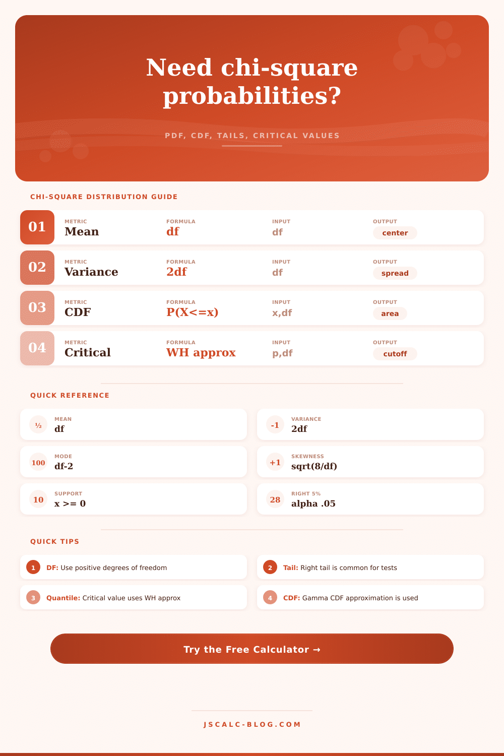
Compute chi-square PDF, cumulative probability, right-tail probability, interval area, distribution moments, and Wilson-Hilferty critical value approximations from degrees of freedom.
🎯Deep Scenario Presets
🧮Distribution Inputs
The context changes wording only; the chi-square distribution math is the same.
Use any positive df. Common tests often use integer df.
Point where PDF, CDF, and right-tail probability are evaluated.
Lower endpoint for P(a < X < b).
Upper endpoint for the interval probability table.
Controls how the Wilson-Hilferty quantile input is interpreted.
Use a decimal probability between 0 and 1, such as 0.05 or 0.95.
Controls displayed PDF, CDF, tail, and cutoff values.
Calculation Breakdown
📌Current Distribution Snapshot
📈Probability Curve at Selected Points
| Point | x value | PDF f(x) | CDF P(X <= x) | Right tail | Interpretation |
|---|---|---|---|---|---|
| Run the calculator to fill the probability table. | |||||
🏁Common Critical Value Reference
| df | Right tail 0.10 | Right tail 0.05 | Right tail 0.025 | Right tail 0.01 |
|---|---|---|---|---|
| 1 | 2.706 | 3.841 | 5.024 | 6.635 |
| 2 | 4.605 | 5.991 | 7.378 | 9.210 |
| 3 | 6.251 | 7.815 | 9.348 | 11.345 |
| 4 | 7.779 | 9.488 | 11.143 | 13.277 |
| 5 | 9.236 | 11.070 | 12.833 | 15.086 |
| 10 | 15.987 | 18.307 | 20.483 | 23.209 |
| 20 | 28.412 | 31.410 | 34.170 | 37.566 |
| 30 | 40.256 | 43.773 | 46.979 | 50.892 |
📚Degrees of Freedom Shape Guide
| df range | Shape | Mean | Variance | Common interpretation |
|---|---|---|---|---|
| 0 < df < 2 | Very right-skewed | df | 2df | Often small-sample or one-parameter cases |
| df = 2 | Exponential | 2 | 4 | Special case with simple CDF |
| 3 to 5 | Strongly skewed | df | 2df | Small contingency or goodness-of-fit tests |
| 6 to 15 | Moderately skewed | df | 2df | Many classroom test-statistic examples |
| 16 to 50 | Milder skew | df | 2df | Variance inference and larger tables |
| Over 50 | Near normal | df | 2df | Normal approximation becomes more reasonable |
🔎Interval and Tail Checks
| Question | Expression | Formula used | Result | How to read it |
|---|---|---|---|---|
| Run the calculator to fill interval and tail checks. | ||||
⚙Formula and Approximation Method
🧪Method Accuracy Checks
| Step | Calculator method | Stable range | Common mistake | Displayed handling |
|---|---|---|---|---|
| Validate df | Require df > 0 | positive df | Using zero df | Warning before results |
| Validate x | Require x >= 0 | support only | Negative test value | Warning before results |
| CDF | Regularized gamma P | most practical df | Using normal CDF directly | Reports gamma CDF label |
| Critical | Wilson-Hilferty transform | best away from tiny df | Forgetting tail direction | Labels WH approximation |
| Interval | F(b) - F(a) | 0 <= a < b | Subtracting tails backward | Sorts endpoints internally |
| Right-tail test | 1 - CDF(x) | 0 to 1 | Comparing CDF as p-value | Shows both CDF and tail |
💡Practical Distribution Tips
For example, maybe you’re testing a new marketing campaign, and you think people respond different depending on where they live. So you gather the results, perform a standard test, and then you have a question: Is the difference I’m seeing due to actual differences between regions; or is it just random noise in my sample?
That’s where the chi-square distribution comes in. This is like a mathematical yardstick. It tells you how far away your observed data has drifted from what you’d expect. The calculator above does all the hard work for you. It takes your raw counts and converts them into probabilities … but what do those probabilities mean?)
What Is the Chi-Square Test?
That’s what the chi-square statistic is: a measure of discrepancy. Specifically, it takes the difference between the observed and expected value, squares those differences, and then scales those squared differences using the expectations. In doing so, it return one number. That’s the cost of the mismatch.
But without some sort of reference point, a number means nothing. That’s where the distribution comes in. It provides a reference point, meaning it offers a way to judge the difference. If your test statistic lands way out on the right tail of the distribution, the mismatch is too big to be explained away as chance. Then you reject the null hypothesis. If it’s closer to center, the data match the model reasonably well.
Here’s the catch: Where does the line get drawn? It’s all about degrees of freedom Degrees of freedom is something that newcomers find confusing. To understand them, consider this. Degrees of freedom represent the amount of independent information you have with which to make an inference about variance.
How do you determine degrees of freedom? Subtract one from the rows and one from the columns, multiply those two numbers together, and then multiply that result by the number of cells in your contingency table. Why does this matter? Once you know the total for most of your cells, the value of the remaining cells are known. In other words, they can’t vary freely anymore.
The more you constrain your degrees of freedom (low number), the more heavily skewed to the right your distribution will be. As you increase the number, the distribution becomes smoother and begins to look like a normal bell curve. If you want to see this illustrated nicely, check out the reference table on the page.
What you’ll notice is that your constraints influences the critical values. The right tail is where most practical uses lie. If you’re doing an independence test, a large deviation will drive the chi-square higher. That shifts it farther to the right on the curve. The smaller the p-value here, the less likely we are to see the data observed given the null hypothesis.
Many people make the mistake here: they mix up which way the tail goes. If your guess is that there’s been less variability than expected, maybe you’re interested in the left tail for your variance test. But for most categorical analysis, it’s the right tail that matters. The right-tail probability and cumulative probability are both calculated by the calculator. You don’t have to wade through thick tables in your textbooks to find these values.
There are some conditions under which the chi-square approximation will not work well. For example, it expects to have at least five observations per cell. If your data is sparse, then you may wish to consider Fishers exact test. It computes critical values with the Wilson-Hilferty approximation. That works really well for moderate degrees of freedom. For small samples, exact methods is safer.
You can see a snapshot of the statistics that describe the distribution (such as the mean, variance and skewness). That gives you an idea how much the data are spread out. A large skewness value means that the distribution has a long right tail (i.e., extreme values is more likely than they would be in a normal distribution).
If you want to use it well, think carefully through the model. What’s your null? How many degrees of freedom do you have? Are your expected counts okay? You should of plugged your statistic into the tool only after those questions. What does it tell you? It will tell you how likely your observed data are under the assumption that the null is true. And if that number is less than the level of significance you’re using (typically 0.05), then you’ve got evidence of either a fit failure or an association between two variable.
It won’t establish causation. It’s no magic bullet. It just measures how surprising something is. But knowing what’s up with the tails and the shape of the distribution lets you read that yardstick propery. You get to judge whether that measure translates to anything meaningful out in the real world.