T Distribution Calculator
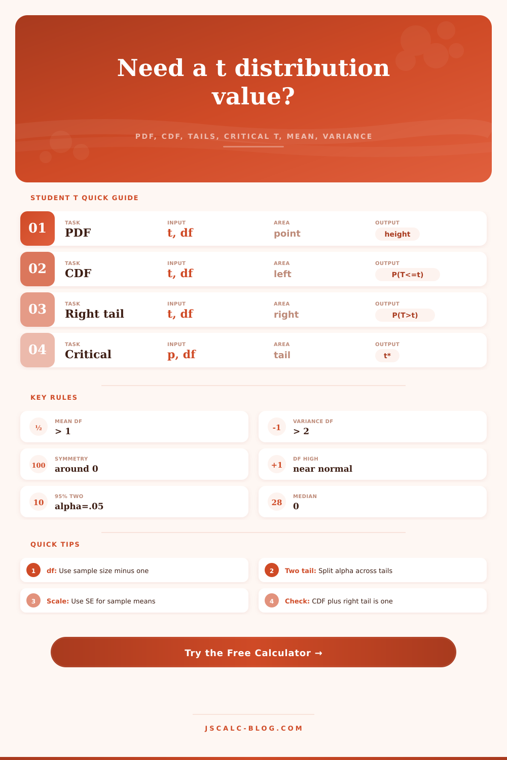
Calculate Student t density, cumulative probability, tail areas, critical values, central intervals, and mean and variance rules from degrees of freedom.
| Degrees of freedom | t 90% central | t 95% central | t 99% central | Shape note |
|---|---|---|---|---|
| 1 | 6.314 | 12.706 | 63.657 | Very heavy tails |
| 2 | 2.920 | 4.303 | 9.925 | Variance undefined |
| 5 | 2.015 | 2.571 | 4.032 | Wide small-sample tails |
| 10 | 1.812 | 2.228 | 3.169 | Common classroom df |
| 20 | 1.725 | 2.086 | 2.845 | Moderate sample |
| 30 | 1.697 | 2.042 | 2.750 | Near normal |
| 60 | 1.671 | 2.000 | 2.660 | Large-sample behavior |
| 120 | 1.658 | 1.980 | 2.617 | Very close to z |
| Calculator mode | What it returns | Main formula idea | Useful when |
|---|---|---|---|
| Left cumulative | P(T <= t) | CDF from regularized beta | Reading a t statistic as a percentile |
| Right tail | P(T > t) | 1 - CDF(t) | One-sided upper-tail tests |
| Two-tail | P(|T| >= |t|) | 2 times the smaller tail | Two-sided significance checks |
| Between | P(a <= T <= b) | CDF(b) - CDF(a) | Central or custom intervals |
| Critical value | t cutoff | Bisection over CDF | Finding test thresholds |
| Mean scale | x-bar interval | mean +/- t* s/sqrt(n) | Confidence intervals for a mean |
In your experiment, you have 12 data points. That’s not a big sample, yet you want to make conclusive claims about larger group that these data points represent. The t distribution stops you from getting too cocky. The normal curve requires you to know the population variance (which is almost never true in actual research). The t distribution handles uncertainty. Your sample standard deviation may or may not be an accurate representation of truth, so it widens the tails of probability. It’s a safer, more truthful approach.
You don’t even need to look up numbers in some mess of tables from your textbooks. The tool does all the complicated stuff for you. All you enter are your degrees of freedom (usually n, 1). Why is that important? Because having less data means the tool penalizes you for it. So if you’ve got twenty observations, then you have nineteen degrees of freedom. Then the tool makes the curve curve accordingly. With fewer degrees of freedom, it results in a flatter curve with heavier tails. With higher degrees of freedom, it produces a sharper curve that looks closer to what we think of as the bell curve. And that is on purpose. It knows that the bigger your sample size, the more closely it estimate true population values.
Why the T Distribution Helps With Small Samples
In testing a hypothesis, we tend to concentrate on the tails, the extreme results, which indicate potential disproving of our null hypothesis. We can select left, right, or two-tails in the calculator. For most scientific questions, the default is two-tailed, since in general you have no idea whether an effect will be positive or negative prior to doing the experiment. So you divide your significance level (e.g., five percent) into two parts, one each end of the distribution. The calculator calculates the area under the curve outside the critical t value. If the observed t statistic occurs in this shaded area, then you reject the null. It’s a yes-no decision based on a continuum of math.
That’s not necessarily bad. In fact, confidence intervals tend to be the most helpful output. Instead of just one point estimate, you recieve a range. That’s what the calculator provides: A range scaled from the critical t value with your standard error. How does that work? Your standard error takes into account the square root of your sample size as well as your sample standard deviation. Intuitively, the bigger your sample size, the narrower the interval; the greater the variance across your data, the wider the interval. However, the width of the interval also depends on the degree of freedom, which protect you from error by making the interval wider when you have smaller sample sizes. Think of it like a buffer from noise.
When you have small sample sizes, the difference between the normal distribution and the t distribution is stark. With only one degree of freedom, the t distribution have heavy tails and technically undefined variance. There is no way to reliably compute your spread. As you work up toward thirty or more degrees of freedom, the difference becomes smaller, but it never dissapears entirely. And it will show you exactly how wide that extra bit is on the calculator. That’s the price of uncertainty.
Know what you’re putting in. You should always make sure you’ve got the right number of degrees of freedom for the type of test design you’re running. A two sample t-test is more complicated because it is based off the variance for each group. For a paired t-test, it is just n, 1. Putting in the wrong degrees of freedom means you’ll have the wrong critical values. Besides entering values for degrees of freedom (and everything else), there are buttons for switching between modes. One mode computes the critical value from a known probability, which comes in handy if you’re planning a study and want to compute how large a sample size would of need to be to see an effect.
The calculator comes with reference tables to provide a quick sanity check. As you move up the degrees of freedom, you can see the critical t value fall. At a ninety-five percent confidence level, it begins at a high value and moves towards the standard normal z-score of 1.96. The closer this gets, the smaller it becomes, reminding you that certainty is not free. Certainty is earned through sample size.
That’s what the t distribution is for: it is a humbling tool, one that reminds us that we’re dealing with limited information, and that there is a sensible structure for communicating its limits. The same logic applies whether you’re assessing quality control metrics in a factory or evaluating clinical trial results. You’ve got a sample, you’ve got some uncertainty, now how do you connect those dots? The calculator will do the arithmetic for you, but you bring the context. Use it to establish your bounds and to describe your risks. Use it to get a sense of what your little bit of data realy tells you. And the broader the tails, the more careful you should be. That is the lesson in every curve.