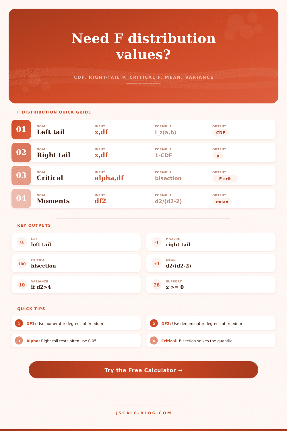
F Distribution Calculator
Calculate left-tail CDF, right-tail p-value, two-tail probability, range probability, mean, variance, and critical F values from numerator and denominator degrees of freedom.
F values are nonnegative. Use 0 for the lower boundary.
Often model, treatment, or numerator variance df.
Often residual, error, or denominator variance df.
Critical F solves P(F > Fcrit) = alpha.
Used for a custom quantile from left-tail probability.
Range probability is P(lower <= F <= upper).
Set this above the lower bound for interval probability.
Affects displayed values only.
Calculation Breakdown
Common Right-Tail Critical Values
| d1 | d2 | F 0.10 | F 0.05 | F 0.01 |
|---|---|---|---|---|
| 1 | 10 | 3.285 | 4.965 | 10.044 |
| 2 | 20 | 2.589 | 3.493 | 5.849 |
| 3 | 30 | 2.289 | 2.922 | 4.510 |
| 5 | 40 | 2.085 | 2.449 | 3.514 |
| 10 | 60 | 1.711 | 1.992 | 2.503 |
| 20 | 120 | 1.459 | 1.665 | 2.025 |
Which F Calculation Fits?
| Use Case | x Input | d1 | d2 | Main Tail |
|---|---|---|---|---|
| One-way ANOVA | MS between / MS within | groups - 1 | N - groups | Right |
| Regression model | MS model / MS error | predictors | N - p - 1 | Right |
| Nested models | extra SS ratio | df difference | full error df | Right |
| Variance ratio | larger s2 / smaller s2 | sample 1 df | sample 2 df | Right |
| Levene style test | reported F statistic | groups - 1 | N - groups | Right |
| Random effects | MS factor / MS error | factor df | error df | Right |
Moment Availability
| Quantity | Condition | Formula | Meaning |
|---|---|---|---|
| Support | Always | x >= 0 | F cannot be negative |
| Mean | d2 > 2 | d2/(d2 - 2) | Expected F value |
| Variance | d2 > 4 | 2d2^2(d1+d2-2)/(d1(d2-2)^2(d2-4)) | Distribution spread |
| Mode | d1 > 2 | d2(d1-2)/(d1(d2+2)) | Peak location |
| Median | Approximation | quantile at p=0.5 | Central cutoff |
Tail Decisions at Common Alpha Levels
| Alpha | Confidence | Right-Tail Rule | Typical Phrase |
|---|---|---|---|
| 0.10 | 90% | p <= 0.10 | Suggestive |
| 0.05 | 95% | p <= 0.05 | Significant |
| 0.025 | 97.5% | p <= 0.025 | Stronger |
| 0.01 | 99% | p <= 0.01 | Very strong |
| 0.001 | 99.9% | p <= 0.001 | Extreme |
So you conduct an experiment, gather some data, get a number and it seems high. Is it noise? Or is it a real signal? This is where the F distribution acts as a kind of guard for our confidence.
No, it’s not merely a curve to memorise. It’s a framework for determining whether difference we’re seeing is real enough to notice.
Understanding the F Distribution
And here’s how it works: You are looking at variance, specifically, you are comparing variances to determine if one group differ from another. So the basic input is an F statistic, a ratio of two variances (in a one-way ANOVA, it’s the ratio of the variance between the group means and the variance with the groups). When the groups is the same, the F statistic will be close to one. A larger than one ratio indicates that most of the variation are due to between-group difference, which is generally what you’re after.
Here’s another thing: the numerator degree of freedom represent variation due to treatment. The denominator degrees of freedom represents variation due to error. Why does it matter? Because the F distribution has a shape that depends on both. If the denominator are bigger, then the distribution itself will be tighter, allowing you to detect smaller effects.
It’s also worth noting that it have a strange tilt on its distribution. While the normal curve begins at zero, the F distribution does not. It is unevenly distributed, starting at zero but skewed to the right. That implies that for small sample size, the critical value tends to be both large (often) and always positive.
If you check the reference table, you’ll note that the critical values gets smaller as you move toward larger degrees of freedom. Why? Because having more data stabilize our variance estimate. With more data, we don’t have to rely so much on such an extreme ratio to assert significance. The calculator accounts for this nonlinearity, allowing it to calculate the exact quantile when degrees of freedom is not multiples of 10 or other common numbers found in standard tables.
It is also noteworthy that when the denominator degrees of freedom is less than 2, the F distribution does not have a mean (in fact, its expected value is infinite). That’s a sign that your sample is so small that you should of not being drawing any conclusions at all. Even more restrictive is rule for the variance of the F distribution, which requires denominator degrees of freedom to be larger than four. Why? Those limits aren’t arbitrary; they’re a reflection of how unstable variance estimates can be in small samples.
By pure luck, you could get an extremely large F value, but it won’t be grounded if you don’t have enough degrees of freedom. Remember: When you interpret the right-tail p-value, what you’re asking is “How probable is it I’d see a ratio this big if the null hypothesis is correct?” If you get a small p-value, then the observed ratio would be unlikely under the null so you’ll reject the null.
But just because you got a big F value doesn’t mean there’s necessarily practical significance. It’s possible you’ve got a tiny effect size but a huge sample which makes the effect stat sig. Context is everything when thinking about your data. The F test answers the question “Is something going on here?”, but it won’t answer the question “Does it matter?”. You need to judge that for yourself, given the size of the differences and the cost of acting/not acting on them.
The point is, the F distribution are a tool for dealing with uncertainty. It provides a systematic approach for measuring how likely something is due to chance versus evidence. From quality control variations to classroom performance to testing a new drug, it doesn’t matter. You measure what’s expected and you measure what’s seen. Then you divide them, and the resulting ratio tell you whether or not your results are reasonable.
The math is simple thanks to the calculator, but understanding what the ratio means is the insight. After all, it boils down to knowing where to draw the line between guessing and believing the numbers.