Central Limit Theorem Calculator
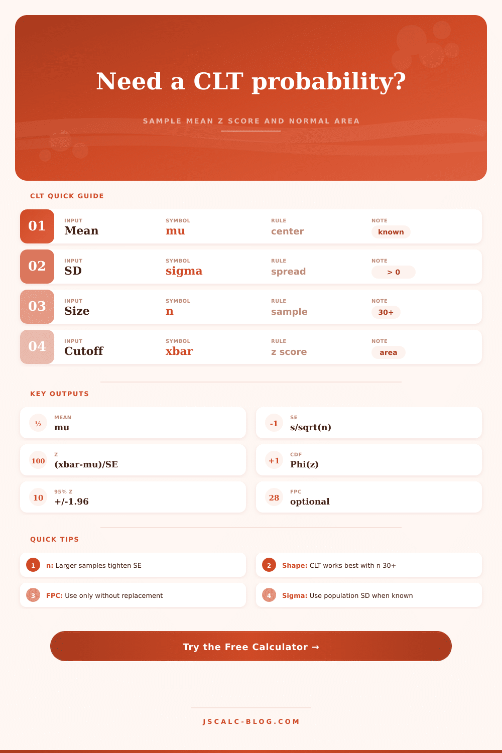
Approximate the sampling distribution of a sample mean with mean μ, standard error σ/√n, z score, normal CDF probability, and optional finite population correction.
🎯Deep Scenario Presets
🧮CLT Inputs
Choose the main probability displayed in card 4.
The expected value of individual observations.
Use the known population SD when available.
The CLT approximation usually improves as n rises.
Used for the z score and one-sided probabilities.
Used for between and outside probabilities.
Use a value greater than the lower cutoff.
Enter 0 to skip FPC; enter N when sampling without replacement.
Calculation Breakdown
📘Sampling Distribution Snapshot
Mean of all possible sample means.
Typical spread of sample means.
Multiplier when sampling from finite N.
Sample size used in the approximation.
Rule-of-thumb approximation quality.
📋Probability Cutoff Table
| Question | Cutoff or range | z value | CDF expression | Probability | Interpretation |
|---|---|---|---|---|---|
| Run the calculator to fill the probability table. | |||||
📈Sample Size Sensitivity Table
| Sample size | Standard error | z at observed x̄ | P(X̄ <= observed) | 95% mean band | FPC status |
|---|---|---|---|---|---|
| Run the calculator to compare sample sizes. | |||||
🔎Central Interval Reference Table
| Central probability | Two-tail alpha | z multiplier | Lower sample mean | Upper sample mean | When to use |
|---|---|---|---|---|---|
| Run the calculator to fill interval cutoffs. | |||||
📚CLT Use Case Reference
| Scenario | Random variable | Typical n | What the mean asks | Watch for | Calculator input |
|---|---|---|---|---|---|
| Quality fill weights | Bottle weight | 30 to 100 | Batch average against target | Drifting equipment mean | Use process sigma |
| Exam score cohorts | Student score | 40 to 300 | Class average above benchmark | Clustered classrooms | Use score SD |
| Delivery operations | Transit minutes | 25 to 200 | Average time beyond SLA | Strong skew or peak windows | Use matching period |
| Survey ratings | Rating value | 50 to 1000 | Mean rating in a finite panel | Nonresponse bias | Add N for FPC |
| Battery testing | Run time hours | 20 to 80 | Mean run time below claim | Small n with skewed failures | Check one-sided tail |
| Call center review | Call minutes | 50 to 500 | Average handle time window | Heavy outliers | Use trimmed process SD if justified |
🔢Formula Method
Sometimes you find that certain groups behave very different than the larger population they are part of. That the sum of several things is drastically different from mean. But then you have stats smoothing out all this craziness. This is all thanks to the central limit theorem. This say that even if your original data is crazy and skewed, averages of large enough samples will fall back on a normal distribution (i.e., This is a bell curve. A bell curve). This principle is basis for nearly every scientific or business statistic test.
Before you do anything else, though, you should of know a bit more about your population. First is the population mean; the true average of what you are trying to estimate. Next up is standard deviation. That tell you how spread out individual data points are. If we’re talking about battery life, for instance, that’s the difference (in hours) between longest-lasting and shortest-lasting devices. Finally, there’s your sample size. The more items you pull into your sample, the smaller standard error will get, meaning the closer your sample mean will be to actual population mean.
Understanding Sample Size and Error
Plug those numbers into the calculator above and it’ll do all the math for you. No need to try to remember coefficients or do any conversions yourself.
One fallacy people have around sample size is they think that by doubling their sample, they cut uncertainty in half. Nope. Standard error depend on the square root of sample size. In fact, to halve the standard error, you must quadruple your sample. That’s a high cost of precision, and that’s why it’s a necessary trade off in terms of how you design your research. What you get with collecting data is what you pay for. Knowing the relationship between these two will help determine whether it’s worthwhile to spend more money to collect more data. It also helps you decide if your sample are enough for the decision you are trying to make.
What if the population you’re sampling isn’t infinite? For example, you might be testing every third light bulb off a short production line. Maybe you’re surveying a small town. In that case, the formulas requires a bit of a tweak. That’s what the finite population correction does: it adjusts the standard error downward. How? Because you’re taking things out of the pool and not putting them back, right? Each item provide you with just a little bit more information than it would if it were in an infinite pool.
This is important when your sample is a large chunk of overall population. Usually this means more than five percent. Ignore it for big manufacturing runs or most web surveys. But pay attention to it for small batches.
Typically, what you care about most is a probability: What’s the probability that my sample mean lies in some range? For this, you are in luck. The z-score let you do this. It tells you how many standard errors your observed value is from the expected mean. If your z-score is large, then under the null hypothesis, your result was rare. The page provides a table showing where your value lands on the normal curve. From there, you can perform tests. You could check whether your new marketing campaign really did move the needle or test quality control limits.
The formulas can be distracting. The intuition isn’t. You’re attempting to filter noise from signal. The central limit theorem provide a map. A calculator provides the destination coordinates. With bigger samples, you decrease noise. It’s not guesswork anymore. It’s measurement. Deviations, extreme or otherwise, becomes measurable. These are decisions that pass muster. That’s the only kind worth making. Eventually, the noise fades away. All that’s left is the truth of the average.