Bootstrap Confidence Interval Calculator
Paste raw observations, choose a statistic, and resample with replacement to estimate percentile, basic, standard-error, and optional normal confidence intervals from the bootstrap distribution.
🎯Deep Bootstrap Presets
🧮Bootstrap Inputs
The same statistic is computed on the original sample and every resample.
Percentile bounds use alpha / 2 and 1 - alpha / 2 quantiles.
Use 1000 to 5000 for stable interactive intervals.
A fixed seed makes the bootstrap run repeatable.
Use percent for percentile or trim; use the original data unit for threshold proportion.
Normal CI is helpful as a symmetric comparison, not always the best interval.
Controls displayed statistics, intervals, and standard error.
Paste numbers separated by commas, spaces, tabs, or line breaks. For binary proportions, paste 0 and 1 values.
📌Current Bootstrap Snapshot
observations parsed
bootstrap draws
split across tails
mean boot minus theta
percentile upper minus lower
📐Formula Breakdown
📊Bootstrap Method Comparison
| Method | Formula | Handles Skew | Best Use | Main Caution |
|---|---|---|---|---|
| Percentile CI | sorted theta_star quantiles | Often yes | Fast nonparametric interval | Can inherit bootstrap bias |
| Basic CI | 2 theta_hat - percentile bounds | Partly | Bias reflection around theta_hat | May invert unintuitive ranges |
| Bootstrap SE | SD of theta_star | No interval alone | Sampling variability estimate | Needs enough B for stability |
| Normal CI | theta_hat +/- z x SE_boot | No | Symmetric benchmark | Weak for skewed statistics |
| Parametric CI | model-based formula | Depends | Normal mean with assumptions | Can fail when assumptions fail |
| Permutation | shuffle labels | Not a CI by default | Null hypothesis testing | Different question than CI |
🧪Statistic Mode Reference
| Statistic | Input Data | Extra Field | Robustness | Typical Question |
|---|---|---|---|---|
| Mean | numeric values | ignored | low | What is the average? |
| Median | numeric values | ignored | high | What is the center under skew? |
| Trimmed mean | numeric values | trim percent | medium | Average after trimming tails |
| Sample SD | numeric values | ignored | low | How variable are observations? |
| Sample variance | numeric values | ignored | low | What is squared-unit spread? |
| Percentile | numeric values | percentile p | medium | What is a tail cutoff? |
| Threshold proportion | numeric values | threshold | medium | What share meets a target? |
🗂Preset Scenario Comparison
| Preset | Statistic | n | B | Confidence | Extra Field | Data Shape | Why Bootstrap Fits |
|---|---|---|---|---|---|---|---|
| Clinic Wait Median | Median | 30 | 2000 | 95% | ignored | right-skewed | Median CI without normality |
| Startup Revenue Mean | Mean | 26 | 3000 | 95% | ignored | lumpy values | Mean under uneven accounts |
| Part Thickness SD | Sample SD | 32 | 2500 | 90% | ignored | tight process | Spread estimate uncertainty |
| Conversion Proportion | Proportion | 40 | 2500 | 95% | 1 | binary | Rate interval from raw outcomes |
| Housing Sale Median | Median | 28 | 3000 | 90% | ignored | skewed price | Robust center interval |
| Delivery 90th Percentile | Percentile | 35 | 3000 | 95% | 90 | tail-heavy | Service tail cutoff interval |
| Plant Growth Trimmed Mean | Trimmed mean | 30 | 2200 | 95% | 10 | mild outliers | Average protected from tails |
| Sensor Variance | Variance | 34 | 2600 | 95% | ignored | calibration drift | Variance uncertainty |
| Exam Score Mean | Mean | 32 | 2000 | 95% | ignored | near normal | SE and normal CI compare well |
| Tickets Above SLA | Proportion | 36 | 3000 | 95% | 48 | thresholded | Share above service limit |
⚙Resampling Quality Checks
| Check | Good Sign | Risk Sign | Why It Matters | What To Do |
|---|---|---|---|---|
| Sample size | n is at least 20 | n below 10 | Tiny samples have few distinct resamples | Report uncertainty cautiously |
| Resample count B | 2000 or more | below 500 | Quantile endpoints can jump | Increase B for final reporting |
| Bootstrap bias | small vs SE | large vs SE | Percentile and normal intervals can disagree | Compare percentile and basic CI |
| Interval shape | percentile near normal | strong asymmetry | Symmetric normal CI may mislead | Prefer percentile or advanced methods |
| Tail statistic | enough tail data | few unique tail values | Percentile stats can be rough | Use more data if possible |
| Independence | one unit per row | clustered repeated rows | Naive bootstrap assumes independent draws | Use cluster bootstrap when needed |
💡Practical Bootstrap Tips
Your data isn’t neatly distributed in some classic form. It’s not a nice, tidy bell curve; it’s a little too messy. And then traditional stats comes along and tells you it won’t work unless your data conforms to certain distributions. It’s as if they’re saying “you’ve got to make this crooked building act straight.”
Bootstrapping doesn’t do that. Instead, it allow the data to speak for itself. Repeatedly. Basically, you resample from your own data, with replacement, thousands of times. The result is a set of simulated datasets that look just as messy (and yet somehow more orderly) then the world you observe.
What is Bootstrapping and How Does It Work?
The calculator above does all behind-the-scenes grunt-work of producing these resamples and calculating the intervals. Now you can spend time figuring out what distribution has to say about how uncertain you really are.
This has a very simple but powerful core: instead of making theoretical assumptions about what “normal” looks like, you use your sample as the closest thing that you have access to for the population. You draw a random sample from your data repeatedly and thereby construct an observed distribution of your statistic. That bootstrapped distribution shows you just how much your estimate could fluctuate if you ran the study again tomorrow. It allows you to quantify the noise, even if you don’t fully know the signal.
The key part here is knowing what it’s really measuring. It’s not variability in the raw data points themselves, it’s variability of the estimate. Choosing the right statistic matters more than the specific method you use to calculate the interval.
If you have skewed data, maybe some very long wait times or high revenues skew your numbers, then the mean can be pulled off-center. It’s better to stick with a median or trimmed mean as an anchor point in these situations. The tool gives you access to many different statistics, such as particular percentiles and variance. This allows you to get that information even if you are more interested in the tails of the distribution than the mean (for example, if you want to know what happens at the worst end rather than the average delivery time).
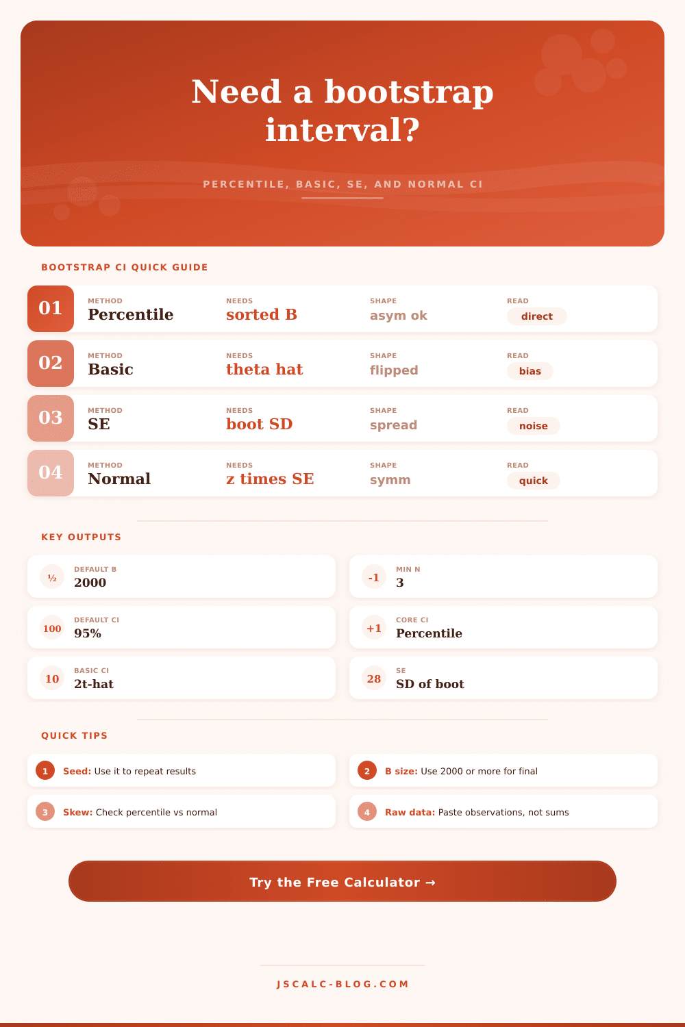
After that, you’re presented with the option of what kind of intervals you’d like. There are a few philosophies behind each one. The most straightforward is called the percentile method. It is just the middle section of all the bootstrap results. It acknowledges asymmetry of your data. If the data allows for it, the interval will extend farther out on one end then the other.
Next, there’s the basic interval, which flips the bounds relative to original estimate. That should help account for any bias in your sampling. And finally, we have the standard error approach. It generates an estimate based off the distribution of bootstrap statistics assuming a normal distribution. This symmetric interval is well-known and fast to calculate. However, it can mislead if your underlying data is highly skewed. Seeing them side-by-side lets you appreciate how much your conclusion depends on the choice of method.
Note how many resamples you run. For a quick look maybe one or a couple hundred is fine. But if you want to pin down your confidence interval endpoints you’ll do better with a couple thousand or even more. The resulting empirical distribution will be smoother; those jaggies on the ends will become smoothed out. This in turn provides tighter boundaries around data.
And one other little detail that’s important for transparency: You use a fixed random seed so that your results can be reproduced. So say you share them with your colleague. They get the same result as you did.
This goes back to the issue of small sample size: How many unique combinations can the bootstrap produce? Small sample sizes mean there are only so many unique combinations available because of a lack of diversity in the data. Resampling from unvaried initial data simply means repeating the same lack of variety. The bootstrap does not invent what’s missing from your observations; it only amplifies what is there. Remember this whenever you see wide intervals derived from tiny data sets.
Bootstrapping, in the end, is all about making peace with uncertainty (not burying our heads in the sand). Simulating the sampling process helps us better appreciate the strength of our estimates. Whether we’re looking at startup metrics or clinical trial data, we should be after the same thing: understanding the range in which the true value most probably lies. And that’s where the calculator gives us the numbers.
But that is also where the wisdom comes in. What do these ranges tell us? What do they mean for our decisions? What does this range of possibilities look like? What can we learn by mapping out this landscape? How does it let us make decisions with just a little less risk? A point estimate becomes a view of possibility. The data is still talking. Now it’s talking a lot more.