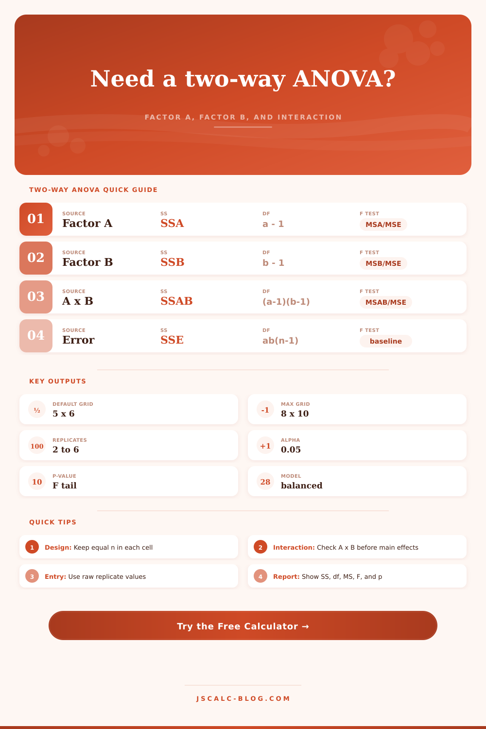
Two-Way ANOVA Calculator
Run a balanced two-factor ANOVA with replication from raw cell observations. The calculator returns SSA, SSB, interaction SS, SSE, degrees of freedom, mean squares, F ratios, approximate p-values, cell means, and formula steps.
🎯 Study Presets
📝 Balanced Factor Inputs
Balanced two-way ANOVA requires the same n in every A x B cell.
Each row is a Factor A level. Separate Factor B cells with vertical bars. Inside each cell, enter the raw replicate values separated by commas.
🔢 Replicate Observations Grid
The default editable grid is 5 x 6. Increase it up to 8 x 10 when your balanced design has more factor levels.
📌 Current Design Snapshot
📊 Calculated ANOVA Tables
P-values use a numerical F distribution approximation from the regularized beta function.
Cell means help reveal whether the interaction is a crossover, a spreading pattern, or mostly parallel shifts.
Marginal means show the average response for each factor level after averaging across the other factor.
📐 Formula Breakdown
🧪 Two-Way ANOVA Source Reference
| Source | What It Tests | Degrees of Freedom | Mean Square | F Ratio |
|---|---|---|---|---|
| Factor A | Average differences among A levels | a - 1 | SSA / dfA | MSA / MSE |
| Factor B | Average differences among B levels | b - 1 | SSB / dfB | MSB / MSE |
| A x B interaction | Whether one factor changes the other factor effect | (a - 1)(b - 1) | SSAB / dfAB | MSAB / MSE |
| Error | Within-cell replicate variation | ab(n - 1) | SSE / dfE | Reference denominator |
| Total | All observed variation around the grand mean | abn - 1 | Not used | Not tested directly |
| Balanced design | Same replicate count in every cell | Required here | Clean SS partition | Standard formulas |
🔍 P-Value Reading Guide
| Result Pattern | Common Reading | Next Comparison | Reporting Focus |
|---|---|---|---|
| Interaction p < alpha | Factor effects depend on each other | Simple effects or cell means | Interaction first |
| A p < alpha only | A levels differ after averaging B | A marginal means | Main effect A |
| B p < alpha only | B levels differ after averaging A | B marginal means | Main effect B |
| No p below alpha | Variation is consistent with noise | Assumptions and power | Effect sizes and CI |
| Large MSE | Replicates vary strongly within cells | Measurement reliability | Error context |
| Tiny MSE | Small within-cell spread | Data rounding or repeatability | Design notes |
💡 Actionable ANOVA Tips
A balanced two-factor analysis of variance lets you test two factors together. In other words: Does your new fertilizer increase yield, and is that good effect lost when you irrigate heavily? One-way tests don’t cut it in such cases; those methods assume the variables does not interact. This tool do the work for you.
Feed it raw data from replicate observations. It will output sums of squares, degrees of freedom, mean squares, and F ratios. You’ll have an idea which (if any) of the factors acts alone, and which are interactive.
How to Use a Two-Way ANOVA Calculator
Make sure you have a balanced design. This means that your design has an equal number of replicates per cell. For instance, if you’re testing how three watering schedules impact your plants when using four different fertilizers (each with three plots for each combination), then you’d need three plots under each remaining pair (in addition to the three already accounted for). Why? A balanced design ensures that the math can neatly separate out the variance.
Since the calculator makes this assumption, your entry grid should reflect it: You’ll be entering actual yield values, not just the average value of the cells. Each individual repeat will contribute to error term, capturing the noise particular to your setup.
What you get back from this is a table that describes what happened. In this case, it’s checking Factor A on the first row and Factor B on the second. The third row is interaction term, which is typically labeled A x B.
You’re not supposed to just look at main effects (which many novices do). You’re supposed to look first at the interaction p-value. That will tell you whether or not effect of one factor depends upon level of the other. If there is an interaction, then the main effects are misleading averages. For instance, a certain fertilizer may look great by itself, but actualy only work well in dry soil while failing in wet soil.
As you add more factor levels, your degrees of freedom shrinks, which you can see in the reference table on the page. But what about the cell means? If the interaction is strong, then you should of look at those means. The calculator gives them to you in a grid, where you can spot the patterns.
Maybe there’s a line on the graph and another line crosses it, indicating a crossover interaction. Maybe the lines spread out, meaning that one factor amplifies the other. That kind of visual intuition doesn’t come through with single F ratio. And the marginal means table help as well.
Even though the interaction may run the story, this table shows you what happens when you average across the other factor. If you look at the bottom of the ANOVA table, there’s the error mean square. This is what your F ratios divide by. If the error term is big, that means either the experimental conditions weren’t stable or your measurements were noisy. If the error term is really small, perhaps your replicates are suspiciously alike, or maybe you’re just rounding your data up to too many significant figures?
Your number of replicates determines how much error your experiments will gets. That number goes into the degrees of freedom shown in the calculator. More replicates gives you more power to detect small effects. But they also take time and money. Before you run any tests or plant anything, you’ll need to make this tradeoff.
The significance level defaults to 0.05, which is typical for most reports in industry and academia. To increase the confidence that your hypothesis is correct, but risk more false negatives (reduce this number). For example, if you’re working with high stakes data and false positives are expensive, you could change it to 0.01. Note that the p-values update automatically as soon as you enter your values.
Below these results is a breakdown of the formulas used to calculate the sums of squares. It reveals the total sum of squares and how it breaks down into its four parts along with a correction factor. For those interested in checking the process or demonstrating it in a report, this gives you a helpful glimpse behind the curtain.
ANOVA is about detecting differences (not size), so even when you get a significant result it doesn’t tell you how big the difference is. That’s something you have to check in the means to judge practical importance.
The calculator does the hard work of summing up the squares and dividing by degrees of freedom, and it provides all the components. Then you apply judgment to determine whether a five percent increase in yield makes the cost of a new fertilizer worthwhile. You decide whether the interaction is a feature or a nuisance.
The data are clarified through the math; what matters is defined by your domain knowledge. This partnership turns data into decisions.