Repeated Measures ANOVA Calculator
Run a one-factor within-subject ANOVA from raw paired scores. The calculator reports treatment, subject, total, and error sums of squares, df, mean squares, F, p-value, and partial eta².
🎯Repeated Measures Presets
📝Within-Subject Inputs
Comma-separated condition names. Every subject row must contain the same number of numeric scores.
Enter one subject per line, with paired scores separated by commas, tabs, semicolons, or spaces.
🔢Current Design Snapshot
📊Repeated Measures ANOVA Table
🧪Condition And Subject Summary
⚙Formula Breakdown
📏Effect Size Benchmarks
| Band | Partial Eta² Range | Percent Of Test Variance | Cohen f Range | Plain Reading | Reporting Note |
|---|---|---|---|---|---|
| Trivial | 0.000 to 0.009 | Under 1% | Under 0.10 | Very little treatment signal | Report if the test is central to the study |
| Small | 0.010 to 0.059 | 1% to 5.9% | 0.10 to 0.25 | Modest within-subject separation | May matter with precise repeated measures |
| Medium | 0.060 to 0.139 | 6% to 13.9% | 0.25 to 0.40 | Clear repeated factor effect | Check pairwise contrasts after the omnibus test |
| Large | 0.140 to 0.259 | 14% to 25.9% | 0.40 to 0.59 | Strong change across conditions | Inspect means and subject patterns |
| Very large | 0.260 and above | 26% or more | 0.59 and above | Treatment dominates residual variation | Verify scaling, outliers, and design coding |
📋Design Check Table
| Check | What The Calculator Assumes | What To Enter | Warning Sign | Result Impact | Action |
|---|---|---|---|---|---|
| Paired rows | Each row is one subject measured repeatedly | Complete subject rows | Missing a cell in a row | Breaks the repeated design | Use only complete paired cases here |
| One factor | All columns are levels of one within-subject factor | 2 or more conditions | Columns mix tasks and groups | F term is no longer one-factor | Use a fuller model in stats software |
| Summary formulas | Sums of squares are computed from raw cell values | Numeric scores only | Percent ranks mixed with raw units | Means and SS become hard to interpret | Keep one measurement scale |
| Sphericity | The displayed F uses uncorrected df | Standard ANOVA data | Many levels with uneven differences | P-value can be too small | Consider corrected df elsewhere |
| Outliers | Subject means and ranges are shown for screening | Rows in original subject order | One subject range dominates | Can inflate or mask effects | Inspect the subject table |
| Reporting | F, df, p, and partial eta² describe the factor | Condition labels in order | Unclear condition names | Hard to reproduce the result | Use descriptive labels |
💡Practical Repeated Measures Tips
Alright, so you’ve done it. You collected data, ran the same subject through three different conditions. You probably measured their reaction time before, during, and after some kind of training intervention. But now what? What do you do to determine whether that change was real or merely due to random chance?
That’s where repeated measures ANOVA enters the scene. By removing the natural variability from one subject to another, it provide a means to strip out noise and isolate effect of your treatment. Simply enter your data into the calculator up top, let it perform the fancy math (summing, dividing…), and you’re left with the answer.
What Is Repeated Measures ANOVA?
But the beauty of this approach is that each participant serves as his or her own control. The issue with a traditional between-groups analysis are that something might be confusing results. Some participants might be older. Others might be naturaly better. Still others might have different temperament. With this design, you eliminate that variation between participants as part of error term. That increases the chance of seeing whether your independent variable is actualy doing anything. It’s akin to measuring someone’s mood at the beginning versus end of a movie instead of comparing moods of two different strangers. You’re interested in how they change, not how they differ different than before.
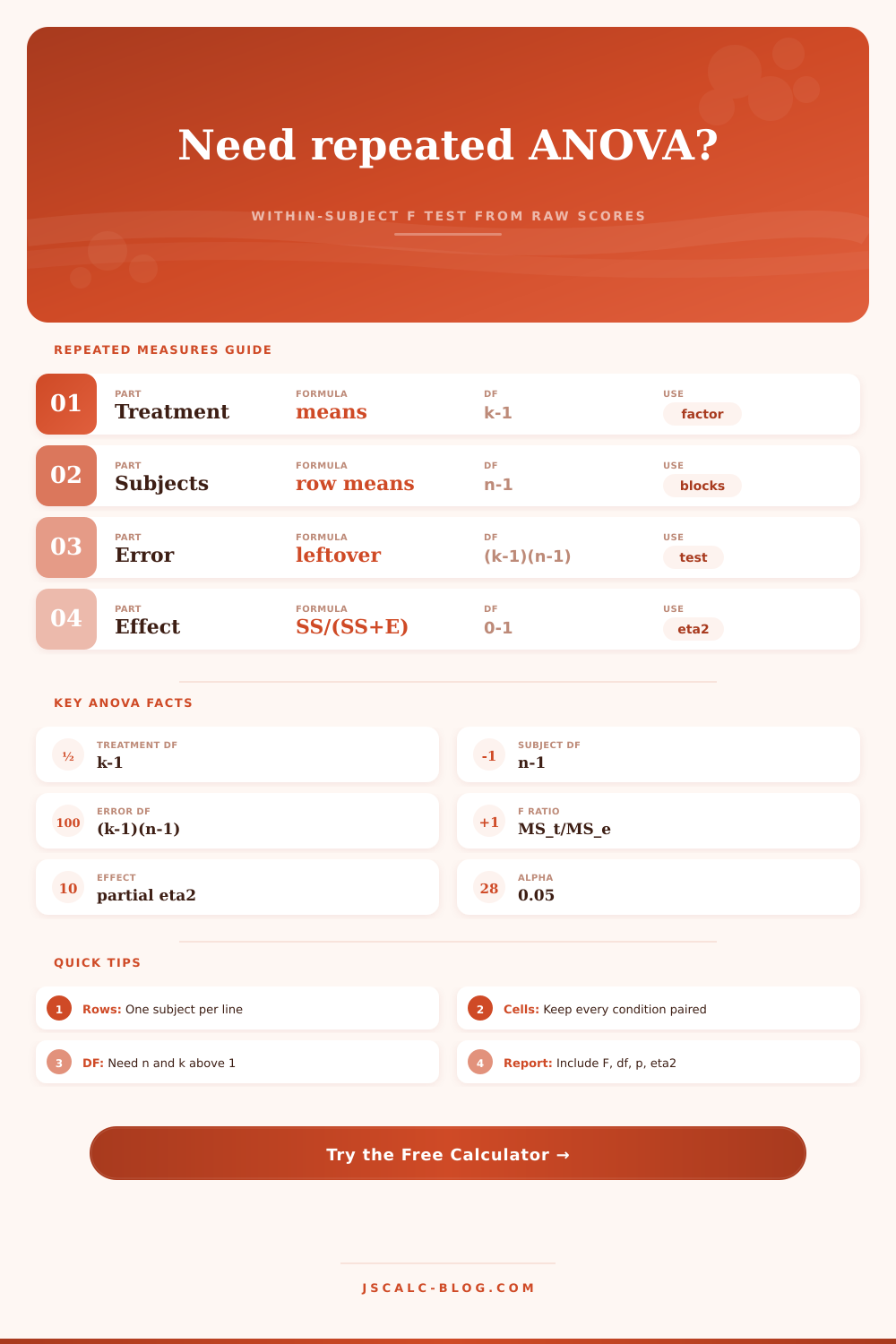
The software divides this up in the following ways: 1) the “treatment” component is effect of interest. 2) the “subject” component (e.g., some people just does better on these tasks than other people). 3) an error component (the unexplained leftover stuff). This is important, as it doesn’t allow individual differences to increase the error spread. That means it provide a more sensitive test.
It outputs an F statistic. That’s a ratio between the mean square for the treatment and the mean square for the error. When the treatment effect are large compared to the residual noise, it’ll have a large value. It also spits out the p-value, which lets you know if the large value has statistical significance.
But don’t stop there. Check out partial eta squared value. This number indicates how much of the variance your treatment explain. It’s called an effect size metric, and can help you understand the practical importance of what you’ve discovered. A statistically significant result with a small effect size could be more of a mathematical curiosity then a meaningful finding.
Keep these critical assumptions in mind. One key one is called sphericity. Sphericity is a statistical condition that states that the variances of the differences between every possible pair of conditions must be equal. When the data doesn’t satisfy this condition, the F test becomes too liberal, which increase your chances of finding a false positive. The tool provides standard uncorrected results, so if you suspect sphericity is violated, you might of need to apply corrections in more advanced statistical package. If you have reason to think sphericity isn’t being met, then you may want to use something like Greenhouse-Geisser to fix your results (in a full-blown statistical package). It’s a common trap for people who just let automated software do everything for them and don’t examine what their data look like.
One note of caution when interpreting these: A statistically significant F test simply indicates that there was some difference between means of at least two conditions. It doesn’t indicate *which* conditions differed. To pin down exactly what’s going on, you’ll probably want to do some sort of follow-up comparison (e.g., planned contrasts, pairwise comparisons).
Also, look in the summary table of subjects. Are there any obvious outliers? One freak score by a subject can realy mess things up. Is it possible the person had an outlier experience and you should investigate whether the result is meaningful? Maybe it shouldn’t be included in your analyses at all.
This is the bottom line. Repeated measures ANOVA is great at picking up differences between treatments (or other conditions) in the same group over time. It also takes advantage of the consistency of responses within subjects to maximize efficiency of your data. If you input your matched pairs carefully and understand how variance breaks down, you’ll be able to make strong conclusions about your experimental variables. This allow you to distinguish between the signal of the treatment itself and the noise of variability among individuals. The test helps you figure out if your results are real or just random noise.