ANOVA F-Statistic Calculator
Calculate a one-way ANOVA F statistic from a completed ANOVA table or from group sample sizes, means, and sample standard deviations. The tool returns SS, df, MS, F, right-tail p-value, effect size, and reporting details.
🎯ANOVA Presets
🧮ANOVA Inputs
Summary mode reconstructs one-way ANOVA from grouped descriptive statistics.
This label changes the result wording only; the F formula is unchanged.
The decision card compares the right-tail p-value with this alpha.
Sorting affects the displayed group contribution table only.
Use 2 or more labels. Commas separate groups; counts, means, and SDs are matched by position.
Enter positive group counts. Decimals are rounded to whole observations.
Means must use the same outcome units across all groups.
Use sample SDs. Within SS is sum((n_i - 1) x SD_i squared).
Used in readable output and tables.
Also called treatment SS, model SS, or factor SS in ANOVA tables.
For one-way ANOVA this is k - 1.
Also called error SS or residual SS.
For one-way ANOVA this is N - k.
Used for context and total N estimate, not the F ratio.
Used in the printable breakdown.
🔢Current ANOVA Snapshot
📋Live ANOVA Table
🧪Group Contribution Table
📐Formula Breakdown
⚖ANOVA Method Comparison
| Input Type | Required Values | Computes SSB | Computes SSW | Best Use | Main Caution |
|---|---|---|---|---|---|
| Group summaries | n, mean, sample SD per group | Yes | Yes | When raw observations are not available but descriptive stats are | Requires sample SD, not SE or population SD |
| Direct ANOVA table | SS_between, SS_within, dfB, dfW | Entered | Entered | Checking published tables or software output | Use the matching error row for the factor |
| Raw data one-way ANOVA | All observations by group | From observations | From observations | Full analysis with residual diagnostics | This page does not store raw rows |
| Repeated measures ANOVA | Subject-level repeated data | Design-specific | Design-specific | Same participants measured repeatedly | Do not use simple one-way independent SS formulas |
| Factorial ANOVA | SS and df for each factor or interaction | Per term | Shared error term | Testing main effects and interactions | Run each term with its correct df and error term |
| Welch ANOVA | Means, variances, and adjusted df | Different method | Adjusted | Unequal variances and unequal group sizes | Classic F table here is not Welch-adjusted |
📏F-Test Interpretation Reference
| p-value Range | Decision at 0.05 | Evidence Wording | F Pattern | Follow-Up |
|---|---|---|---|---|
| Below 0.001 | Reject H0 | Very strong evidence group means differ | Between MS far above within MS | Run planned contrasts or post-hoc tests |
| 0.001 to 0.009 | Reject H0 | Strong evidence of at least one mean difference | F is clearly above 1 | Check effect size and assumptions |
| 0.010 to 0.049 | Reject H0 | Statistically significant at 5% | F large for its df pair | Report F(dfB, dfW), p, and eta squared |
| 0.050 to 0.099 | Do not reject at 5% | Suggestive but not conventional | F may be moderately above 1 | Avoid strong claims; review power |
| 0.100 to 0.500 | Do not reject | Weak evidence against equal means | F near 1 or modest | Inspect design, variance, and sample size |
| Above 0.500 | Do not reject | Observed group differences fit random variation | F often near or below 1 | Summarize uncertainty and practical size |
📊Preset Reference Table
| Preset | Groups | Total n | Outcome | Input Style | Expected F Pattern | Typical Reading |
|---|---|---|---|---|---|---|
| Teaching Methods | 6 | 116 | Score points | Means and SDs | Moderate F | Classroom method differences |
| Fertilizer Trial | 5 | 60 | Yield kg | Means and SDs | High F | Fertilizer treatments separate clearly |
| Landing Pages | 6 | 360 | Conversion percent | Means and SDs | Small F | Variant means are close |
| Therapy Groups | 4 | 92 | Symptom score | Means and SDs | High F | Treatment group mean shift |
| Machine Output | 6 | 144 | Part weight g | Means and SDs | Moderate F | Machines need process review |
| Department Salaries | 7 | 217 | Salary k | Means and SDs | Very high F | Department means are not equal |
| Lab Batches | 8 | 96 | Assay value | Means and SDs | Low F | Batch means mostly align |
| Training Programs | 5 | 150 | Productivity index | Means and SDs | Moderate F | Program differences worth follow-up |
| Direct Small ANOVA | 4 | 48 | Outcome units | SS and df | Moderate F | Manual table check |
| Direct Published Table | 6 | 180 | Outcome units | SS and df | Strong F | Published ANOVA row verification |
🔍Assumption and Reporting Checklist
| Check | Good Sign | Risk Sign | Why It Matters | What To Report |
|---|---|---|---|---|
| Independence | Each observation belongs to one group | Repeated or paired measurements | Classic one-way ANOVA assumes independent errors | Sampling and assignment design |
| Variance similarity | Largest SD is not much larger than smallest SD | Large SD ratio with uneven n | F test can be sensitive to heteroscedasticity | SDs by group and any Welch backup |
| Normal residuals | Residual plots are roughly symmetric | Strong skew or heavy tails | P-value accuracy relies on model residuals | Diagnostics or robust method if needed |
| Degrees freedom | dfB = k - 1 and dfW = N - k | df copied from the wrong ANOVA row | F p-value depends directly on both df values | F(dfB, dfW) |
| Effect size | Eta squared reported with p-value | Only significant or not significant wording | Practical meaning needs a size estimate | eta squared or omega squared |
| Follow-up tests | Contrasts planned or adjusted post-hoc tests | Many unadjusted pairwise tests | ANOVA only says at least one mean differs | Contrast method and adjustment |
💡Practical ANOVA Tips
Does the average difference between groups matter? Or was it simply random noise? With one-way ANOVA, you can find out. This compares all the groups at once. Unlike pairwise comparisons where you might compare each group with every other this method avoids leaving you prone to a false positive in any additional comparison.
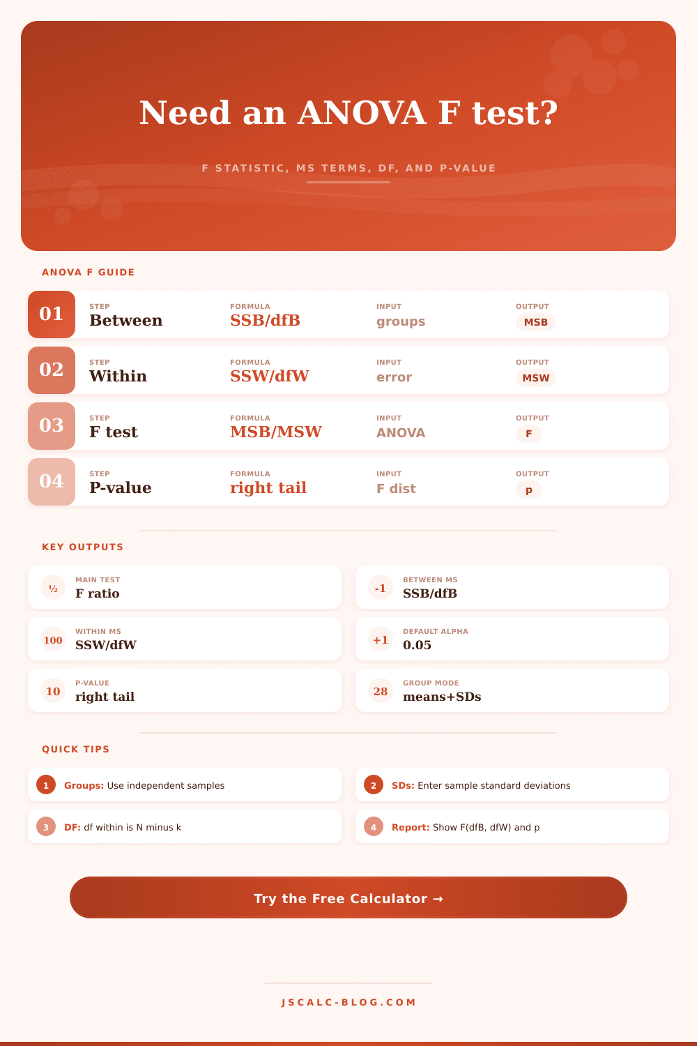
So the null hypothesis is that each group’s mean are equal. How do we know? It breaks down like this: there are two sources of variation. There’s the variation within each group; representing the normal scatter of your data points. And there’s the variation between group means which gives you reason to think your treatment may be doing something. If the between-group variation is much greater than the within-group variation, then you’re seeing signs that something systematic are happening. The F statistic is the ratio of these two variances.
How One-Way ANOVA Works
Give the calculator your summary stats and let it do the heavy lifting for you. Getting a valid output requires knowing what goes into the model. For a start, most users enter in the summary mode (with mean, standard deviation, and sample size per group). Note that we are entering the sample standard deviation, this is different than the standard error of the mean. The latter shrinks as sample size increase. If entered here, it will falsely increase the F ratio and make results appear more significant then they actually are.
Based off these values, the tool calculates the sum of squares for both the between-group and within-groups terms. Dividing those sums of squares by their corresponding degrees of freedom generate mean squares. Degrees of freedom equals the number of independent pieces of information used to estimate variability. So if there are 3 groups, then that becomes n-1 for the between-groups term; and n-(n/3) = n-1 for the within-groups term. The denominator adjust the variance estimate to make it a fair comparison across samples of different sizes/groups… Whether small or large.
From there, you want to know if this F ratio represent something statistically significant. For that, you look at the p value. This tells you the likelihood of getting this F statistic (or higher) by chance if your null hypothesis was correct. In other words, the lower the p value, the less likely it is that the results could of occurred just by random chance. So you’re looking for a small p value. You then compare this against some chosen cutoff (typically).05 (to decide what’s going on). If the p value is smaller than this cutoff, you can say that the differences between the means are probably not due to chance alone and you’ll reject the null hypothesis. At least one of the group mean is different from another group mean.
This is where many folks misunderstand things; they think this test lets you know which groups differ. It doesn’t. A significant overall test simply indicates that not all means are equal, meaning you’ll want to run some sort of post hoc test or planned contrast to identify the specific differences. The chart on this page show the different p-value ranges and how strong the evidence is for each. It also shows what you should do next.
Before taking the numbers at face value though, it’s also good to check your assumptions. For example, ANOVA requires the data to be independent, and the variances in each group to be approximately equal. If the groups have different sample sizes (especially if one has a much greater spread), the F test may be unreliable. You may need a non-parametric alternative or some sort of Welch adjustment for this.
Eta squared is another measure provided by the calculator: it shows how much of the total variance are explained by the differences between groups. Why? Because statistical significance doesn’t necessarily imply practical importance. With a huge sample size, a tiny difference could be found to be statistically significant, whereas even a large difference wouldn’t with very few observations. Reporting the p value along with the effect size paints a far fuller picture of what you’re looking at.
In short, the point is to split out signal from noise in an interpretable and rigorous fashion, which applies whether you’re contrasting fertilzer treatments, teaching methods, or the outputs from machines. You want to know what portion of the variation you see is due to the experimental factor, versus the remainder of variation that’s always going to be there, in the background of your data. The tool makes the math easy, but the thinking is on you. Did you find a difference big enough to make a difference in the real world? It is not just in some statistical table. You must think that through.
Careful attention to the inputs and careful interpretation of the outputs, turns a pile of numbers into an indication that at least one group is different: Are these groups really different? It is a small thing, but it matters.