ANOVA Sum of Squares Calculator
Compute one-way ANOVA sums of squares from group summaries. Enter each group's n, mean, and sample SD to get the grand mean, SSB, SSW, SST, mean squares, F ratio, and eta squared.
Load a realistic grouped-data scenario, then edit the n, mean, SD, labels, precision, and reporting focus.
Enter at least two groups to calculate ANOVA sums of squares.
This changes interpretation text only; the SS formulas stay the same.
Calculations use full precision; this only formats the displayed result.
Examples: score, yield, response time, conversion rate, weight, rating.
Leave blank for unitless data; SS and MS are in squared units.
Default uses the requested within formula: sum(n_i - 1)s_i^2.
Sorting affects the detail table only; totals are unchanged.
Highlights related rows in the comparison and formula tables.
Enter one group per line. The three numbers are sample size, group mean, and sample SD unless you switch to sample variance.
| Group | n | Mean | Spread | Mean - Grand | Between SS Part | Within SS Part |
|---|---|---|---|---|---|---|
| Enter group summaries to see SSB and SSW contributions. | ||||||
| Source | SS | df | MS | Formula | Interpretation |
|---|---|---|---|---|---|
| Between groups | 0 | 0 | 0 | SSB / (k - 1) | Variation explained by group means |
| Within groups | 0 | 0 | 0 | SSW / (N - k) | Residual variation inside groups |
| Total | 0 | 0 | 0 | SSB + SSW | Total corrected variation around grand mean |
| F ratio | 0 | dfB, dfW | MSB / MSW | F = MSB / MSW | Needs positive MSW |
| Eta squared | 0 | proportion | SSB / SST | Effect size | Share of total SS explained by groups |
| Quantity | Uses | Depends On | Common Mistake | Report Wording |
|---|---|---|---|---|
| Total SS | All corrected outcome variation | Every observation and grand mean | Using raw sum of squares instead | SST = sum(x - grand)2 |
| Between SS | Variation from group mean differences | n_i and each group mean | Ignoring unequal group sizes | SSB = sum n_i(mean_i - grand)2 |
| Within SS | Residual variation inside groups | n_i and sample SD or variance | Using n instead of n - 1 for sample SD | SSW = sum(n_i - 1)s_i2 |
| Mean squares | Scale SS by degrees freedom | SSB, SSW, dfB, dfW | Comparing raw SS when df differs | MSB = SSB / dfB; MSW = SSW / dfW |
| F ratio | ANOVA signal strength | MSB and MSW | Calling F an effect size | F(dfB, dfW) = MSB / MSW |
| Eta squared | Variance share effect size | SSB and SST | Reporting without model context | eta2 = SSB / SST |
| Preset | Groups | Total N | Response | Pattern | Typical Reading |
|---|---|---|---|---|---|
| Teaching Methods | 3 | 88 | test score | ordered means | clear between-group signal |
| Fertilizer Trial | 4 | 64 | plant yield | best treatment high | large experimental effect |
| Reaction Time Lab | 3 | 72 | reaction time | small SDs | strong mean separation |
| Production Lines | 5 | 100 | part weight | tight process spread | quality-control comparison |
| Hospital Units | 4 | 152 | length of stay | unequal n | moderate unit differences |
| Ad Creative Test | 4 | 960 | conversion rate | large samples | small but measurable lift |
| Reading Programs | 3 | 81 | fluency gain | school intervention | medium learning effect |
| Battery Batches | 4 | 60 | runtime | batch variation | manufacturing stability check |
| Support Teams | 4 | 172 | minutes to resolve | unequal teams | service-time comparison |
| Training Blocks | 5 | 125 | skill score | progressive means | large training separation |
It is not necessary that you eyeball all of the individual data points to decide whether or not your groups differ. Most analysts gets stuck in the weeds of spreadsheets. They manually calculate differences until it get mind-numbingly boring.
Enter group summaries into this calculator. Then let it crunch some numbers. There is no chance of an arithmetic mistake so you will get a clear indication of whether your experiments produced significantly different results.
How to Understand Your Data Results
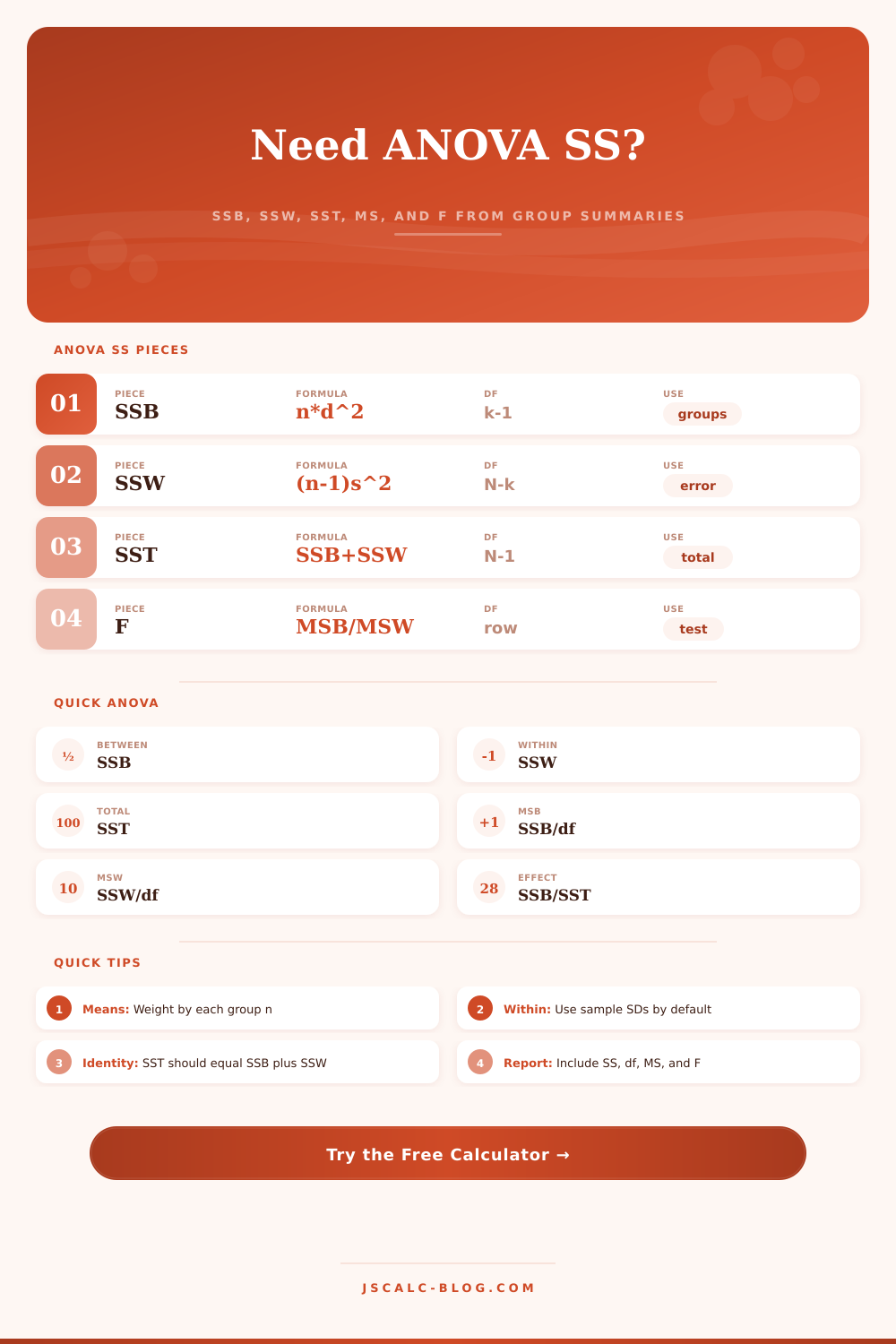
Analysis of variance works by breaking down the total variation into two pieces. The first piece is the variation between groups (between means for each group). The second piece is the variation within each group. If the between-groups variation is substantially greater then the within-group variation, then you’ve got a signal. If they’re roughly equal in magnitude, then your observed differences are probably nothing more than noise. You must understand what these pieces represent so that you know how to interpret the result.
First let’s examine the between-group sum of squares. It represents the distance between each group’s average and the overall grand mean. What most people mess up on here is that the grand mean need to be weighted based off sample size. A group with ten people doesn’t count as much toward the grand mean as a group with fifty. The tool does that math for you. That way the distance it’s calculating for the between-group variance will be correct. If you just average the groups’ means (without using weights) then you’ll skew your estimate. This is what most analysts screw up on in their quick mental check.
Now think about the within-group sum of squares. It’s the noise or error that’s built into your data. To compute it, you need the sample standard deviation of each group. Plug those numbers in and the formula account for the degrees of freedom within each group. As the page explains, all these pieces fit together with the reference table on the same page. When you input your standard deviations, you’re informing the model just how much a score varies from its own group average. If there’s high variation among individuals within groups then weak between-group signals gets drowned out.
Finally, we have the F ratio. To find the F ratio, divide the mean square between by the mean square within. So if your group differences are big compared to the amount of noise in your data then you’ll get a big F ratio. Don’t mistake a big F ratio for a big effect size. You can have a very small difference between your groups but still get a massive F ratio because you’re dealing with such a big sample size.
That’s why the tool also provides eta squared. Eta squared tell you what proportion of all the variation in the data is due to your grouping. It puts a scale on the effect that the F ratio does not convey alone. So many people get hung up on significance. Did I find a statistically significant result? What they fail to consider is, so what? Maybe the difference in my test scores between two adult-sized sofa was only half a point. Sure that’s statistically significant, but does it matter? The sums of squares show you just how big the results are. It puts some context into your end results. How much of the variation is explained by random chance or by the groups?
So this is what I mean: imagine it’s a story of your data. The means are the center of the groups. The standard deviations are the amount by which the data spreads out. And the sample sizes are the weight you should of given each group. When you put all those together, then you have a full picture of whether your interventions produced different results.
You don’t need to memorize the algebraic formulas behind each component. Just understand that there’s variation everywhere, and that your task is to filter signal from noise. That’s what the tool does for you. It helps you decide whether the differences you observe are substantial enough to alter your decision.
Statistics isn’t about discovering some magic number. It’s about measuring uncertainty. Knowing precisely how much of the variation stems from your treatment versus randomness let you make decisions with your eyes open.