Post Hoc Tukey Calculator
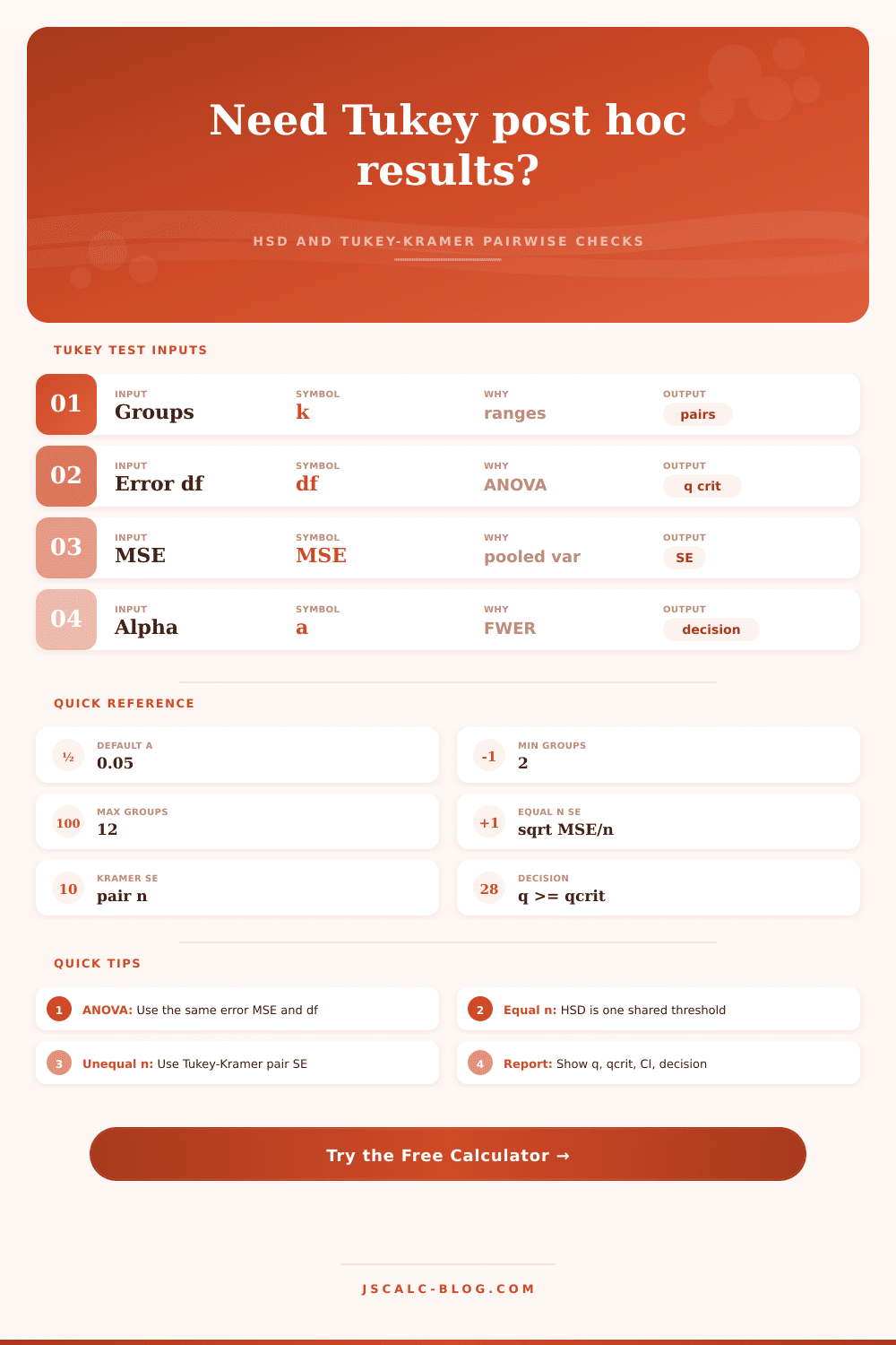
Compare all group means after ANOVA with Tukey HSD for equal sample sizes or Tukey-Kramer pairwise standard errors for unequal sample sizes.
Enter 2 to 12 labels. The calculator uses the first k labels and creates missing labels automatically.
Means must use the same response scale as the ANOVA that supplied MSE and df_error.
For equal-n HSD, the single equal sample size controls the SE. For Tukey-Kramer, each listed n_i is used pair by pair.
| Pair | Mean diff | SE | q statistic | q critical | Approx adjusted p | Simultaneous CI | Decision |
|---|---|---|---|---|---|---|---|
| Results load when the calculator runs. | |||||||
| Rank | Group | Mean | n | Distance from grand mean | Best-group gap |
|---|---|---|---|---|---|
| Group summaries load when the calculator runs. | |||||
Equal n Tukey HSD: HSD = q_alpha(k, df_error) × sqrt(MSE / n). Any absolute mean difference at least this large is flagged significant.
Tukey-Kramer: SE_ij = sqrt(MSE / 2 × (1 / n_i + 1 / n_j)); q_ij = abs(mean_i - mean_j) / SE_ij; compare q_ij with q_alpha(k, df_error).
q approximation label: Browser JavaScript has no built-in studentized range quantile. This calculator approximates q_alpha from a familywise-adjusted t quantile and reports that method in every breakdown.
| Alpha | Familywise confidence | Pairwise alpha used | q critical approximation | Equal-n HSD | Decision impact |
|---|---|---|---|---|---|
| Critical values load when the calculator runs. | |||||
| Situation | Recommended setting | Standard error | Decision rule | What to report |
|---|---|---|---|---|
| Equal sample sizes in every group | Equal n - Tukey HSD | sqrt(MSE / n) | abs(diff) >= HSD | HSD, q, qcrit, adjusted p |
| Unequal but independent group sizes | Unequal n - Tukey-Kramer | sqrt(MSE / 2 x (1/ni + 1/nj)) | q_ij >= qcrit | Pair SE, q, qcrit, CI |
| Only two groups | Post hoc test is unnecessary | Same as pooled t | Equivalent to one comparison | Use the original planned test |
| ANOVA error term is not shared | Do not use Tukey HSD | Needs a common MSE | Check model assumptions first | Consider Games-Howell |
| Very unequal variances | Tukey is fragile | Pooled MSE may mislead | Welch-style post hoc preferred | Report the variance issue |
| Many groups and small df | Expect larger qcrit | Same formula | More difficult to reject | Show alpha and df_error |
OK, you’ve run the analysis of variance and the F-test is significant. So you know your groups aren’t all the same. But you don’t want to inflate your error rate by finding out which groups differ from each other! That’s why you use a multiple comparison procedure like Tukey test, which controls the familywise error rate: the probability of making at least one false discovery over all pairwise comparisons. And it doesn’t just stop you from fishing for significance; it does the math for you.
All you need to plug into calculator are your means and error terms. You will no longer have to look up values manually or deal with rounding errors creeping in because you’re in a rush. Enter all those values into input phase. Patience is required. Enter the degrees of freedom and mean square error as they come from your initial ANOVA. Don’t make up new error terms. Don’t pull out an error term from some other experiment’s pooled variance. MSE is your system’s level of noise. That’s the variance that was left over after explaining what’s different between groups.
How to Use the Tukey Test Calculator
High MSE? This results in big standard errors. You need a larger mean difference to call it significant. The calculator uses this level of noise to construct the confidence intervals.
Note: Unequal sample sizes are fine, just flip to the Tukey-Kramer method. Classic Tukey HSD assumes equal n. This makes the standard error very simple, one common value for all. For unequal sample sizes, every pairwise comparison gets its own standard error calculation. Smaller groups contributes more uncertainty. Tool handles this automatically, adjusting the denominator for each comparison. No need to balance the precision of Group A vs. B in your brain.
The other choice is which alpha level you choose. That’s your preference for the tolerance to false positives. Zero point zero five is default. That’s what most fields use. For something more serious, such as drug approval, you could go down to zero point zero one. That would be very strict. The calculator changes the critical q value for that. The lower the alpha, the tighter the bar to reach statistical significance. So there will be fewer significant pairs. No big deal. It is just the price of certainty. The reference table on the page explains where those levels fall. It also shows how much more stringent they make it to reject the null hypothesis.
There’s no free lunch. You can’t have perfect sensitivity and perfect specificity.
But the fun part comes next: interpreting the output table. For each pair, pay attention to the q statistic. That’s the observed difference expressed as multiples of its own standard error. So if the q in the column is greater than the critical q in the row, then the difference is statisticaly significant.
Remember: Statistics aren’t the same as importance; they’re statistics. Even a small difference can be important if you have a very small MSE (error term) and a large sample size. Always check out the mean difference itself. Is a 5 point difference between test scores something meaningful in class? Maybe not. A 2 millimeter difference in material strength might not be strong enough for a bridge.
The calculator outputs the simultaneous confidence intervals. Those represent the range of plausible differences. If the interval spans zero, then you don’t have a difference. If it does not span zero, you do. And that interval will get wider or narrower based on your sample sizes and your error term.
There’s an important bit of nuance that people miss with the Tukey-Kramer adjustment. It protects you against false positives. It’s conservative. But it’s also hard on your power. For example, if your groups are really uneven in size, you’ll get large confidence intervals around the pairs that involve smallest group. You may not catch a real difference there. It is not a bug. It is a feature. You’re paying for protection against false discoveries.
Don’t try to hack it and remove some data points so you end up balancing the groups. That introduces bias. Live with the wider intervals for the underrepresented groups. The method is strong. It’s not magic. You can’t make signal out of noise.
The presets on tool are good sanity checks. Load a fertilizer trial or a study on teaching methods and see what the numbers do with real world data. Get an idea of the scale of the output. Note that for designs with equal n, the HSD threshold is just one number. For unequal n there is a set of different thresholds. The decision rule is the same. Compare the statistic vs the critical value. You either reject or fail to reject. Means are ranked at group level. Helps you see the lay of the land. Biggest gap is often easiest to spot. The smallest significant gap is the most interesting. Tells you where boundary of your effect lives.
The bottom line is that post hoc testing is exploratory. In other words, you didn’t anticipate these exact comparisons ahead of time. You’re searching for patterns. With the Tukey method, you have a way of safely doing so. It keeps your error rate honest. Use it to inform your next experiment. Use it to compose your report. Know that the probability provided by the calculator isn’t the truth itself. You must still interpret findings within the context of your field. Those numbers provide the map; you’re the one walking the territory.