One-Way ANOVA Calculator
Compare three or more independent group means from summary statistics. Enter each group as label, sample size, mean, and sample standard deviation, then review the grand mean, ANOVA table, F statistic, p-value from the F CDF, and eta² effect size.
🎯ANOVA Presets
🧮Group Summary Inputs
Use one group per line. Commas, tabs, semicolons, or vertical bars are accepted between the four values.
The decision card compares the right-tail p-value with alpha.
Use more decimals when reporting small p-values or close decisions.
Sorting changes the display table only, not the ANOVA math.
This is a quick screen, not a formal homogeneity-of-variance test.
The benchmark label is descriptive; eta² itself is unchanged.
🔢Current ANOVA Snapshot
📊Live Group Contribution Table
⚙Formula Breakdown
📋ANOVA Table Structure
| Source | Sum of Squares | Degrees Freedom | Mean Square | F Ratio | P-value Role |
|---|---|---|---|---|---|
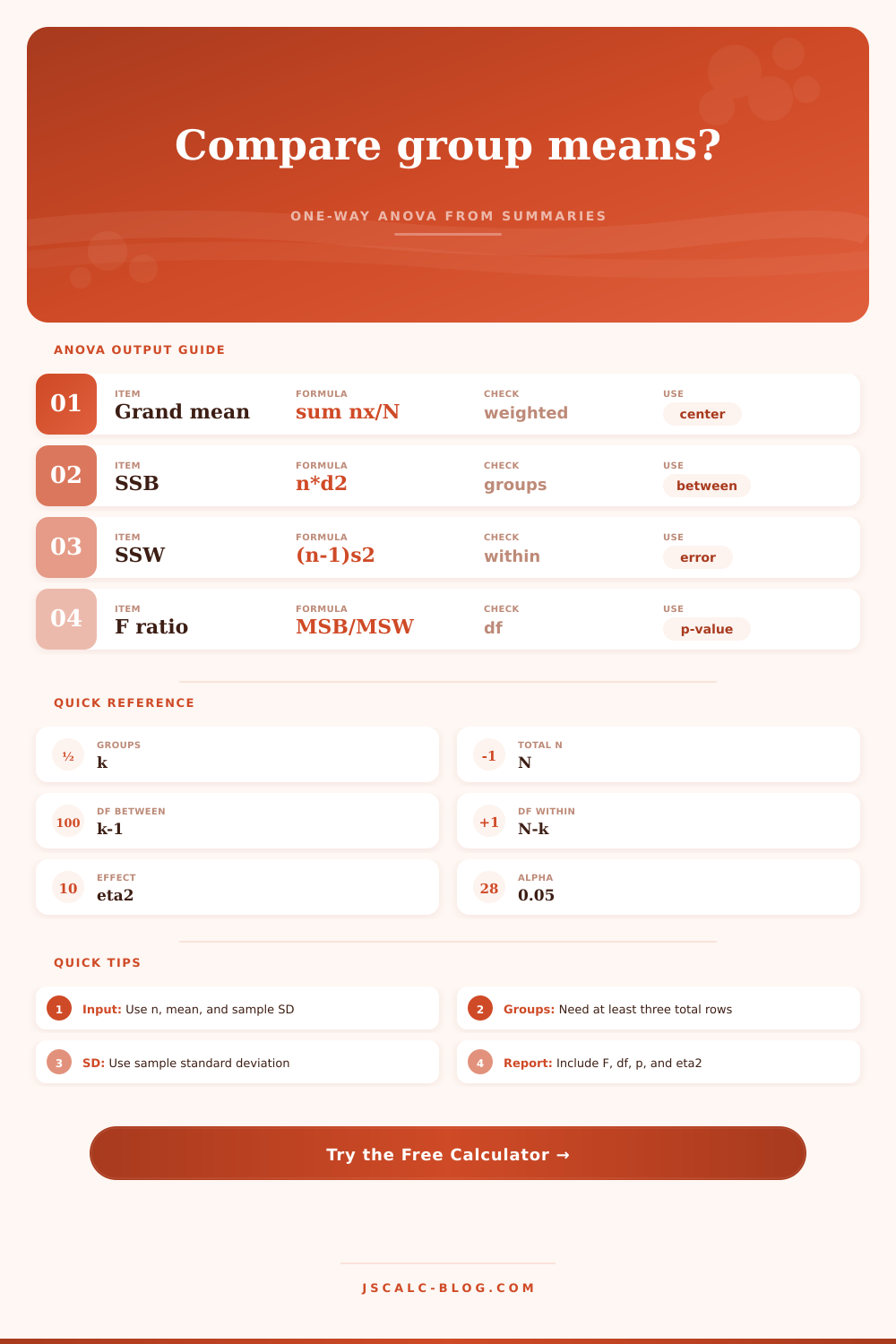
| Between groups | sum ni(mean_i - grand mean)^2 | k - 1 | SSB / df_between | MSB / MSW | Numerator of F test |
| Within groups | sum (ni - 1)si^2 | N - k | SSW / df_within | Reference error | Denominator of F test |
| Total | SSB + SSW | N - 1 | Not used directly | Not applicable | Denominator for eta squared |
📏Eta Squared Benchmarks
| Band | Eta Squared Range | Variance Share | Cohen f Approx. | Plain Reading | Reporting Note |
|---|---|---|---|---|---|
| Trivial | 0.000 to 0.009 | Under 1% | Under 0.10 | Group means explain little variation | Still report if hypothesis driven |
| Small | 0.010 to 0.059 | 1% to 5.9% | 0.10 to 0.25 | Detectable but modest separation | Context matters more than the label |
| Medium | 0.060 to 0.139 | 6% to 13.9% | 0.25 to 0.40 | Clear group-level difference | Useful for planning follow-up work |
| Large | 0.140 to 0.259 | 14% to 25.9% | 0.40 to 0.59 | Strong practical separation | Inspect assumptions and outliers |
| Very large | 0.260 and up | 26% and up | 0.59 and up | Group membership dominates variation | Verify design and measurement scale |
🧪Preset Input Reference
| Preset | Groups | Total n | Outcome Example | Mean Pattern | Variance Context | Typical Reading |
|---|---|---|---|---|---|---|
| Teaching Methods | 3 | 85 | Exam score | Lecture to workshop rises | Similar SDs | Medium teaching effect |
| Fertilizer Yield | 4 | 96 | Yield per plot | Treatment C highest | Moderate SD spread | Large treatment signal |
| Ad Creative Test | 5 | 1,120 | Conversion rate index | Variant D strongest | High precision | Small but testable lift |
| Assembly Lines | 4 | 180 | Output per hour | Line 4 lower | Uneven SD screen | Investigate line process |
| Dosage Groups | 4 | 128 | Symptom score | Dose response shape | Clinical summaries | Clear dosage effect |
| Onboarding Flow | 3 | 760 | Activation score | Guided highest | Large samples | Reliable mean separation |
| Class Sections | 6 | 174 | Quiz average | Small section spread | Balanced enough | Modest classroom variation |
| Lab Temperature | 5 | 100 | Reaction time | Curved response | Similar SDs | Strong condition effect |
| Training Plans | 4 | 92 | Performance gain | Coached plan highest | Small-sample screen | Practical training difference |
💡Practical ANOVA Tips
One way ANOVA exist to solve your multiple comparisons problem by considering all groups simultaneously. The difference between group isn’t really what it’s measuring; it’s measuring signal to noise ratio. The calculator do that math for you (above), but how do you interpret what its telling you?
What is it measuring? There is variance. Variance is the amount of total variation in your score. So what you do are divide that up into two kinds of variation: 1) How much does the variation between your groups matter? This is called “signal.” This measures how far away the group means fall on average from the overall average.
How to Use One-Way ANOVA
2) How much does the variation within your groups matter? This is called “noise” or “error,” and it measure how much individuals vary from their own group mean. The F-statistic is just signal over the error. Basically if the grouping factor is meaningful, then the groups should of been pretty different than one another relative to how similar student inside each group are. In other words, a big number implies the grouping factor matter.
Most projects fail at the input phase. For example, the calculator request the standard deviation of sample (of each group). This is NOT the same thing as the standard error. Standard deviation do not change based off sample size. The standard error decreases as the sample size increases.
Plugging in the standard error mean your F-value will be overstated. You’ll think something is significant when it’s not. Double-check your inputs against original data. Is the value beside the mean small? Are you sure it isn’t precision but rather spread?
The tool can handles varying sample sizes and weights itself accordingly. To avoid letting smaller groups influence center point, it computes a grand mean that takes into account how large each group is.
In these kinds of test, assumptions matter more then in others. One of those is that the variance among the groups are about the same. That’s often a fair bet if you’re testing in a controlled laboratory setting. But that is not the case when comparing a big corp account to a little startup.
There’s a handy screen on the calculator for that. It alerts you to biggest standard deviation divided by the smallest. If that ratio gets too high, the F-test become unreliable and you might need a Welch adjustment or a transformation. The tool will tell you the numbers. You’ll have to eyeball whether the spread seem OK given your context.
The p-value doesn’t tell the story of effect size. If you have a huge sample, it’s possible for the p-value to be statistically significant despite a tiny effect; conversely, with a tiny sample, even a huge effect can fail to reach statistical significance. That’s where eta squared comes into play.
It fills the gap. Eta squared reports the proportion of variance explain by your groups. One indicates the groups explain everything; zero indicates they add no information. Somewhere in-between is where you’ll land in the real world. Social science is full of small effects, while physiology are full of big effects (that said, knowing where your field typically lands will help you understand the result).
Get disciplined about reporting. Include in your report the following: F-value, df (degrees of freedom), p-value, effect size. There are actualy two kinds of degrees of freedom. One is the total sample size minus the number of groups. The second depend on how many group you have. Those two variables tells you the shape of the distribution and what level of difference is significant. All those values are clearly given by the calculator. Simply cut-and-paste them into your report.
That applies everywhere, as the tool’s presets demonstrate: Marketers use it for their ad clicks. Manufacturers use it for assembly lines. And teachers use it for exam scores. It is the same math in a different context.
Remember to ask whether your differences has any practical meaning. Practical significance is a spectrum; statistical significance is an all-or-nothing choice. Look at the spread, check out the means, decide if it’s worth changing your strategy.
The beauty of one-way ANOVA is that it’s a pretty robust workhorse. Even if you have slightly uneven sample size, it works through them; even if your data isn’t perfectly normally distributed, it’s OK-ish; you get a single test to clear then you can look around for outliers, run some post-hoc tests, or refine the model. You need that initial test though to warrant searching around.
That’s where the calculator come in. It takes your messy summary and creates a clear decision point: did I clear the hurdle? The key is knowing exactly what you’re measuring, and the rest follows from there.