Contingency Table Calculator
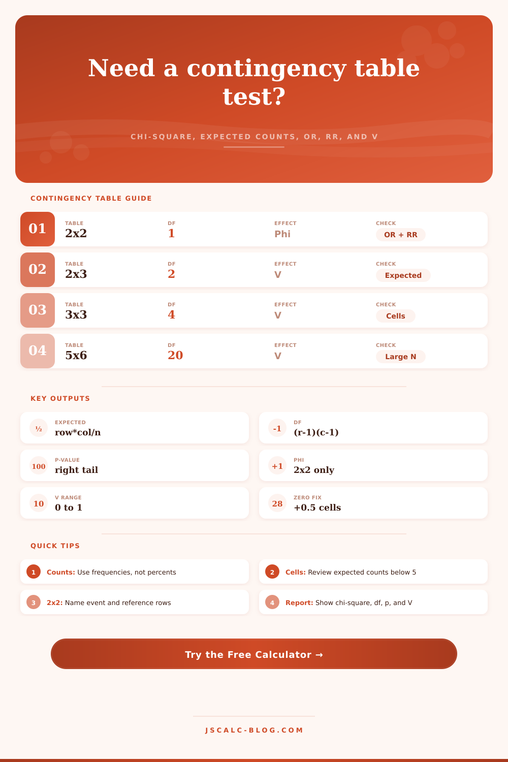
Enter a 2x2 or RxC frequency table to calculate row totals, column totals, expected counts, chi-square, degrees of freedom, p-value, and association strength.
📌 Presets
⚙ Table Setup
🧮 Diagnostic Grid
📋 Observed Counts and Totals
🔢 Expected Counts
🔍 Chi-Square Contributions
📐 Method Reference
| Output | Formula | Use | Applies To | Null Value |
|---|---|---|---|---|
| Expected count | (row total × column total) / N | Independence model cell count | Any RxC table | Observed = expected |
| Chi-square | Sum (O - E)² / E | Overall departure from independence | Any RxC table | 0 |
| Degrees of freedom | (rows - 1)(columns - 1) | Reference distribution shape | Any RxC table | Not a test value |
| Phi | (ad - bc) / sqrt(r1 r2 c1 c2) | Signed association direction | 2x2 only | 0 |
| Cramer's V | sqrt(chi-square / (N × min(r - 1, c - 1))) | Association strength from 0 to 1 | 2x2 or RxC | 0 |
| Odds ratio | (a × d) / (b × c) | Odds comparison between rows | 2x2 only | 1 |
| Risk ratio | [a / (a + b)] / [c / (c + d)] | Risk comparison between rows | 2x2 only | 1 |
✅ Practical Checks
Is there a relationship between two things? That’s the basic question you begin with. Did a medical treatment improve outcomes? Was a marketing email responsible for driving sales? This is the type of question researchers and product managers asks to separate their findings from their hunches.
That separation comes in the form of a contingency table, which is where the chi-square test for independence works. A count table is just a grid of counts. On one axis it has your categories (e.g., control vs. Treatment group) while the other axis shows your outcomes (e.g., recovered vs. Not recovered).
What Is a Chi-Square Test?
The table of raw numbers appear straightforward, yet they’re easily misleading. More is always better… And thus bigger groups has more events simply by virtue of being bigger. Absolute counts don’t help you compare groups. Instead, you need to adjust them to what you’d expect based off the absence of any relationship.
This is something many do not do. They only look at the observed data, ignoring expected data. The calculator does that math for us. It creates the grid and computes the marginal totals. And it determine what the count in each cell ought to be based on idea of independence. Where the observed count is way off from the expected count, you’ve got something. Where they’re close, you’ve got silence.
All those differences are summed into the chi-square statistic. The higher the number, the more the data don’t match the independence model; so, the lower the number, the more they does.
What’s driving the test? Degrees of freedom act as an engine. These factors determine how much variation can occurs in the data. They also determine what distribution we use to evaluate your chi-square score. For example, a two-by-two table has only one degree of freedom. As you add more columns and/or rows, you increase degrees of freedom. Each additional degree of freedom require a higher chi-square score to be significant. You cannot compare scores across tables with varying numbers of degrees of freedom.
To do so, you must look at the p-value. That will tell you probability of randomly encountering the pattern. When it is lower than your pre-set threshold (typically five percent). You’ll call it a relationship.
That is important because strength is not significance. It is a fundamental distinction. If your sample size is large enough, even a small association can be statistically significant. To understand the connection, you require effect size measures. For two-by-two tables, phi and odds ratios indicates both the magnitude and direction. For larger tables, Cramer’s V normalizes the association on a scale from zero to one. The closer it gets to one, the more perfect the prediction; at zero, there is no link. Reporting a p-value without an effect size is like reporting speed without units; you have the number, but you lack the context.
You’ve got the number. But what does it mean?
There are pitfalls with this procedure. Insufficent amounts of data in any one cell will lead to problems using the chi-square approximation. Typically you should of had at least five observations per cell. When it’s less than that, the test isn’t reliable. The calculator notes this and offers an adjustment.
Alternatively, if some cells contain zero, it prevents calculation of the odds ratio because you cannot divide by zero. In such cases, a small constant is added to make the math smooth. Analysis continue even though the data may be sparse.
The key to understanding what happened are the contributions. Which cells is driving that chi-square? Is there a huge overrepresentation of something in one category, or a slight change all around? This is the diagnostic piece that converts a yes/no response to a story. It points you to the action.
Statistics follows a common sense structure: statistics is just structured common sense. You have a hunch about whether something is random or real. And the contingency table provide an unbiased way for you to ask that question. Define your categories. Count up your observations. Let the math do the work.
What’s the verdict? Is there an association or not? You begin with a hunch; you conclude with a finding. The numbers tell you truth.