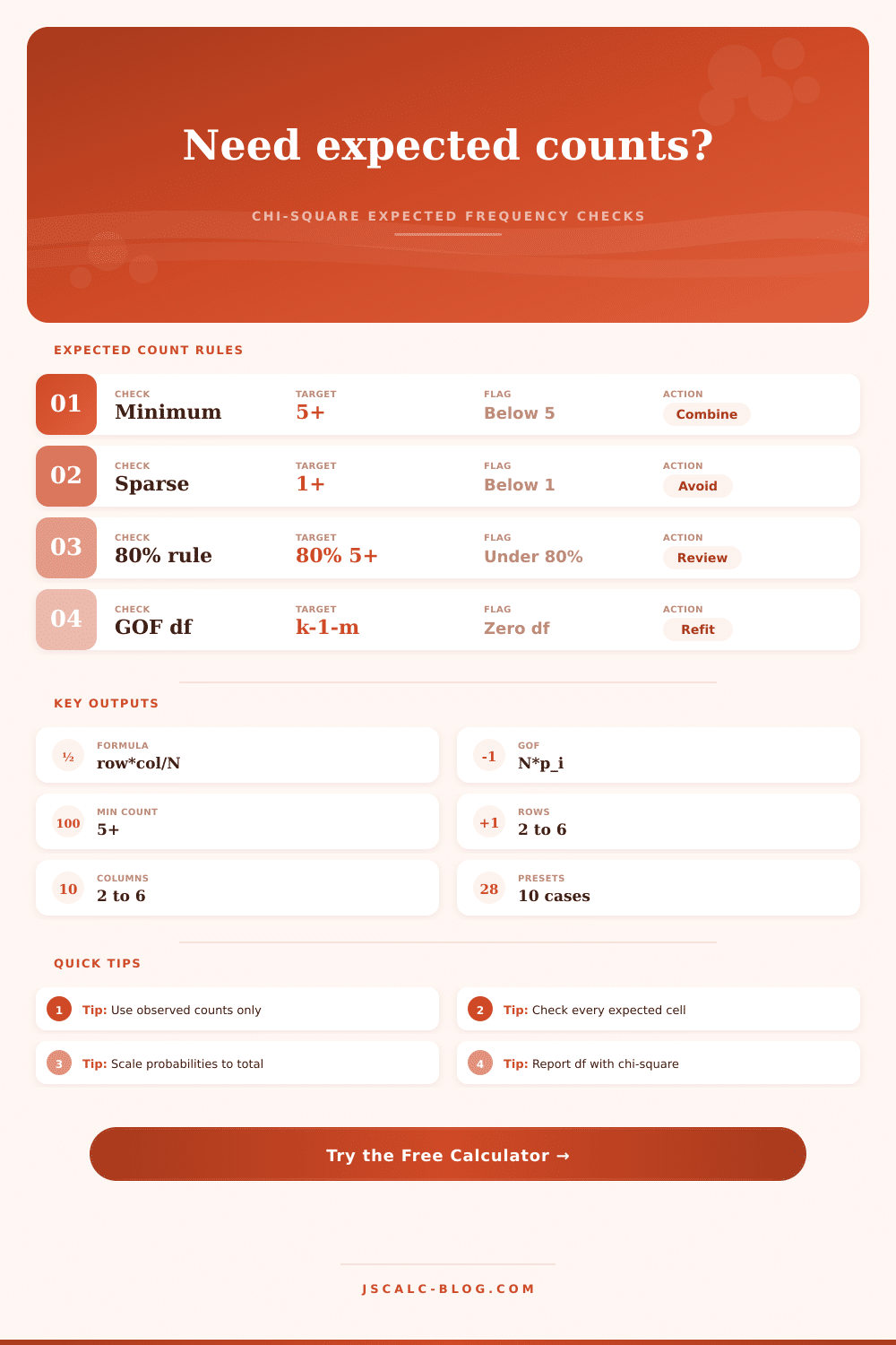
Chi-Square Expected Frequency Calculator
Find expected frequencies for chi-square independence and goodness-of-fit tests, compare observed counts, and screen every cell against the common minimum expected count rules.
📌Expected Frequency Presets
🧮Chi-Square Inputs
Independence uses row and column totals. GOF uses total count times expected probability.
The calculator still computes expected counts when a rule is flagged.
Use more decimals when totals are small or probabilities are uneven.
Use contributions for chi-square totals; use residuals for direction.
Rows are the first categorical variable or sample groups.
Columns are outcomes, choices, categories, or conditions.
Comma-separated labels. Blank labels become Row 1, Row 2, and so on.
Use short labels so expected-frequency tables stay readable.
Paste rows with commas, tabs, spaces, or semicolons. These are observed frequencies, not percentages.
Enter counts in category order. The observed total is used as N.
Comma-separated labels aligned with the observed counts.
Ratios are normalized into probabilities before E_i = N x p_i.
Length must match the observed category list. Every expected weight must be positive.
Use 0 for fixed probabilities; use 1 or more if parameters were estimated from the same data.
Expected frequencies are always scaled to the observed total for the test.
🔢Expected Count Snapshot
📋Observed Counts Table
Expected Frequencies
Cell Diagnostics
📐Formulas Used
✅Expected Frequency Rule Table
| Screen | Common threshold | Why it matters | Calculator flag | Typical response | Best use |
|---|---|---|---|---|---|
| Classic minimum | Every expected count at least 5 | Protects the chi-square approximation | Any cell below 5 | Combine defensible categories or use exact methods | Small to medium tables |
| 80 percent rule | 80% of cells at least 5 and none below 1 | Allows limited sparsity in larger tables | Too many cells below 5 | Inspect sparse rows and columns | Larger exploratory tables |
| Planning screen | Every expected count at least 10 | Adds margin before data collection | Any cell below 10 | Increase sample size or reduce categories | Study planning |
| Severe sparsity | No expected count below 1 | Very small expectations distort the test | Minimum below 1 | Avoid asymptotic chi-square reporting | All count tables |
| Zero margin | No zero row or column totals | Expected cells become zero | Zero total row or column | Remove empty categories before testing | Data cleaning |
| GOF probability | All p_i positive and sum to 1 after scaling | Each category needs an expected frequency | Missing or zero weight | Fix the model probabilities | Goodness-of-fit |
📊Chi-Square Test Comparison Grid
| Test setup | Observed input | Expected formula | Degrees of freedom | Minimum count check | What to report |
|---|---|---|---|---|---|
| Independence | Two-way count table | row total x column total / N | (r - 1)(c - 1) | Every expected cell | X², df, p, expected-count warning |
| Homogeneity | Groups by outcome table | row total x column total / N | (r - 1)(c - 1) | Every expected cell | Same as independence |
| Goodness-of-fit | One count list | N x expected probability | k - 1 - fitted parameters | Every category expected count | X², df, p, model probabilities |
| Equal proportions GOF | One count list | N / k for each category | k - 1 | Every category expected count | Counts and equal-share model |
| Fitted model GOF | One count list plus fitted model | N x fitted p_i | k - 1 - fitted parameters | Every category expected count | Subtract fitted parameters from df |
| Large sparse table | Many row and column groups | row total x column total / N | (r - 1)(c - 1) | 80 percent rule may be reviewed | Expected-count caveat and table shape |
💡Practical Tips
Look at the contingency table. You observe that more people in treatment group have recovered than in control group. Your intuition tell you this means drug is effective. But your intuition doesn’t consider chance, especially not small samples, especially not unbalanced ones. So how can you know whether the pattern you’re seeing isn’t just luck?
That’s what you need to test against: the hypothetical situation of no treatment effect at all. That is the expectation, or expected frequencies. It anchors the chi-square tests to reality.
Understanding Expected Frequencies in Chi-Square Tests
The calculator above will run math for you, but understanding what it is doing matter more than clicking the button. The expected frequencys in an independence test aren’t guessed at. They are calculated using marginal totals. This produces a mathematical answer for what would be expected if there were no relationship at all between your variables. To calculate it, multiply row total by column total. Then divide by grand total. Do that for every cell and you have created a model of pure randomness.
When the observed counts comes close to matching the expected values, the chi-square statistic stay small. The bigger the difference between the two, the larger the statistic becomes. This indicate a possible real association. Compare reality to a null world.
Goodness-of-fit tests work a little differently. Here you’re not trying to compare two variables. Rather you want to see whether your data fit some particular kind of distribution (a fair die; a 3:1 ratio of genes). To figure that out, it multiplies probability for each category times the overall sample size. So with a fair die, we expect to see every face come up one-sixth of the time. If our observed count doesn’t match this expectation then the test says the fit is bad.
Expected counts must also be positive. Probabilities should adds to one. The calculator will automaticly adjust your inputs so you don’t have to worry about scaling your percentages yourself.
One caveat that pops up among statistics students has to do with cell counts. Each cell should ideally contain at least five observations. It’s not a recommendation; it’s a way to protect against using an estimate. Why? Because the chi-square test rely on the sampling distribution being approximately normal. That doesn’t hold when expected frequencys get too small. So, the resulting p-value may mislead you.
To accommodate lower numbers, some researchers relax the requirement as long as no cell contain less than one observation and at least 80% of cells exceed five. It’s a balance between being practical and being thorough. For sparse data, a tough rule ensures you won’t falsely reject the null hypothesis. If your table is huge but a couple cells are small, easy-going rule lets you keep the entire dataset.
Why do we need residuals? Residuals tell you how actual data differ from what was expected. When the null hypothesis is true (and expected frequencies are based off that), the actual counts will be close to those expectations. If you see a big positive number for a residual, it means there were more than chance would predict; if a big negative number, less then predicted by chance.
The total chi-square tell you that something happened different, but doesn’t tell you where. That’s what the residuals tell you. In a drug trial, for example, the overall effect may have been significant, but looking at the residuals you find that only people of a certain age benefited from treatment.
Never merge just because it makes the numbers look better! Yes, merging sparse cells is fine… provided that resulting categories make sense. For example, combining “mild” and “severe” just to get the five-count rule isn’t okay. You’re hiding something important. You should of used more data.
This tool will highlight where the cells might be an issue. Then, consider: Is it worth getting slightly more accurate numbers at the cost of less detail? In many cases, no. Better to go back, tweak your categories or gather additional data first.
It’s simple mathematics, but it takes skill to interpret it. The “expected” column shows what happens if there is no real difference: This is what you’d expect if your hunch turned out to be wrong. Does your data differ significantly from that expected frequency? Then you’ve got some evidence. Is it clustered around the expected? Then you’ve got nothing but noise.
Look at minimum counts. Check the residuals. There’s still time to run through the hypothetical table and test if your pattern holds up… Or if it was all a matter of chance.