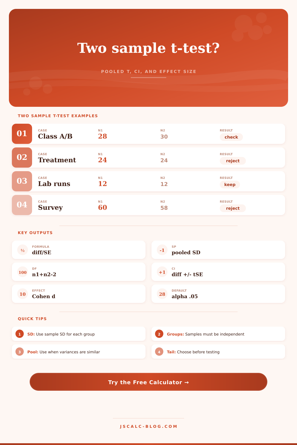
Two Sample T-Test Calculator
Compare two independent sample means with the pooled two sample t-test: t = (mean1 - mean2) / (sp * sqrt(1/n1 + 1/n2)), pooled standard deviation, df = n1 + n2 - 2, p-value, confidence interval, and Cohen's d.
📌Presets
Load an independent two-group comparison, then adjust means, sample standard deviations, sample sizes, tail, confidence level, and alpha.
Enter two independent sample summaries to calculate the pooled two sample t-test.
⚙Test Inputs
🔢Calculated Quick Grid
📋Pooled T-Test Reference Tables
| Check | Use pooled test when | Watch out when | Useful number | Next step |
|---|---|---|---|---|
| Independence | Observations are from separate people, items, or runs. | The same subject appears in both groups. | paired data | Use paired t-test instead. |
| Variance similarity | Sample SDs are close enough for a pooled variance model. | One sample SD is much larger than the other. | ratio > 4 | Compare with Welch's t-test. |
| Sample size | Both groups have at least two observations and no empty cell. | A group is tiny and skewed. | n1, n2 >= 2 | Inspect raw values if available. |
| Normality | Data are roughly normal, or samples are moderately large. | Strong skew or heavy outliers drive the mean. | n near 30 | Use plots or robust checks. |
| Direction | The alternative hypothesis was chosen before analysis. | Tail is picked after seeing the sign. | left/right/two | Report the planned tail. |
| Interpretation | p-value, CI, and effect size are reported together. | Only the reject/keep decision is reported. | d and CI | Use all outputs. |
| df | One-tail 0.10 | One-tail 0.05 | One-tail 0.01 | Two-tail 0.05 | Two-tail 0.01 |
|---|---|---|---|---|---|
| 10 | 1.372 | 1.812 | 2.764 | 2.228 | 3.169 |
| 20 | 1.325 | 1.725 | 2.528 | 2.086 | 2.845 |
| Output | Formula | Meaning | Report cue | Common caution |
|---|---|---|---|---|
| Pooled SD | sp = sqrt(((n1 - 1)s1^2 + (n2 - 1)s2^2) / df) | Shared within-group standard deviation estimate. | Show sp when using pooled t. | Needs similar variances. |
| Standard error | SE = sp * sqrt(1/n1 + 1/n2) | Expected sampling spread of mean1 - mean2. | Used in t and CI. | Gets smaller with larger n. |
| t statistic | t = (mean1 - mean2) / SE | Signed distance from zero difference in SE units. | Include df with t. | Sign depends on group order. |
| Confidence interval | diff +/- t* x SE | Range of plausible true mean differences. | Check whether zero is inside. | CI is two-sided here. |
| Cohen's d | d = (mean1 - mean2) / sp | Mean difference in pooled SD units. | Report magnitude and sign. | Context matters. |
| Decision | Reject H0 if p <= alpha | Formal alpha-based test result. | Pair with p-value. | Not a practical-size measure. |
🧮Formula Notes
Imagine you are trying out a new way of teaching, splitting one half of the class up and teaching them one way while leaving the other half alone. The next day, you give everyone the same test. You get some different results, now how do you know which one was better? Now we look at statistics.
For this problem, the typical solution is the two sample t-test. This asks you to believe your data enough to pool the variance. Most people stumble here, because they don’t think their data justifies the assumption. Pooling variance give you more statistical power, but it also means you take on some risk of being incorrect about your assumption. This means you assumed that the groups had similar spread.
How to Use a Pooled Variance T-Test Calculator
In short, this page’s calculator performs the arithmetic to calculate the pooled variance. It spits out an effect size, a confidence interval, the p-value, and the t-statistic all at once. This makes it easy to see what happened so you can concentrate less on crunching numbers.
Let’s start by explaining what pooling standard deviations even accomplishes in the first place. Running a t-test involve taking the difference in two means and assessing how large the difference is compared to the noise (i.e., “background variation“) within the data. By adding together the two groups’ standard deviations, you get a better estimate of this background noise if the two groups has approximately the same amount of variability in their population. In other words, it’s similar to combining your best guesses from multiple good sources, instead of having only one source.
The formula for degrees of freedom is N1 + N2, 2. Why? Because this adjusts for your task of estimating two means with the data. If your samples is small, these missing degrees of freedom become quite important. They’ll increase the width of the confidence interval and reduce your ability to claim significance.
But before entering in any numbers, first check the variance ratio. If one group is wildly more spread out than the other, then the pooled approach may mislead. You can consider this rule of thumb: Look at the ratio of the larger variance and divide by the smaller. Then, if the ratio is greater than four, then you may want to use Welch’s t-test. Why? Because that test doesn’t assume equal variances.
The tool here includes a check on the variance ratio as part of its output grid. It helps you validate your choice of test. If the ratio is low, you’re safe to go ahead and use the pooled method. But if it’s high, then the p-value you get may well be inaccurate. And you can end up being led down a path to false conclusions. It’s a little diagnostic step, but it keeps you from making some serious errors.
Set your inputs and then understand the output. First, what does the p-value mean? Does it mean the difference is important? No. Does it say that the difference isn’t important? Again, no. The p-value only indicates if the difference is statistically significant or not.
That’s why we look at Cohen’s d next. This value measures the effect size, or the distance between the two means in standard deviations. In other words, it expresses the mean difference in units of standard deviation. If you have a massive sample size and obtain a tiny p-value, it doesn’t necessarily mean the difference is big. It may be really small but still be statistically significant. On the flipside, you might get a non-significant p-value in a small study and miss a big and important effect entirely. By looking at both together, the calculator lets you see the whole story.
Report the confidence interval, too. Why? Because it tells you a possible range of plausible differences between the groups. If this interval contains 0, it means you could potentially have no difference whatsoever.
Picking the tail direction based off what you see in the data is a common mistake. Looking at the means first can lead you to pick a one-tailed test (to increase your p-value). That’s gaming the system. You should of defined the alternative hypothesis prior to analyzing and collecting the data. When you’re exploring things, a two-tailed test is safer. It protects you from bias in either direction. You can use the tool to select the tail type.
Planning matters. The software doesn’t matter. The quality of the result depends on how well you planned it.
A second pitfall is ignoring the assumption of independence. Are the groups dependent? Do they contain some of the same subjects? If so, then the groups are dependent, and you need to do something other than pool their variances. Dependent data violates the very logic of the test.
Finally, keep in mind that statistical significance is not the same as practical importance. Statistical significance doesn’t always mean the result matters. And lack of statistical significance might still suggest something. This binary outcome, to reject or not reject the null hypothesis, is only half the story. Be nuanced in your understanding. Consider the confidence interval and effect size. These inform your ability to assess the precision and size of your results.
The calculation is done for you by the calculator. The judgment part is yours. Combine thoughtful interpretation with rigid mathematics, and you transform raw numbers into actionable insights. This is how you shift from merely calculating a t-statistic to truly understanding what your data reveals.