One Sample T-Test Calculator
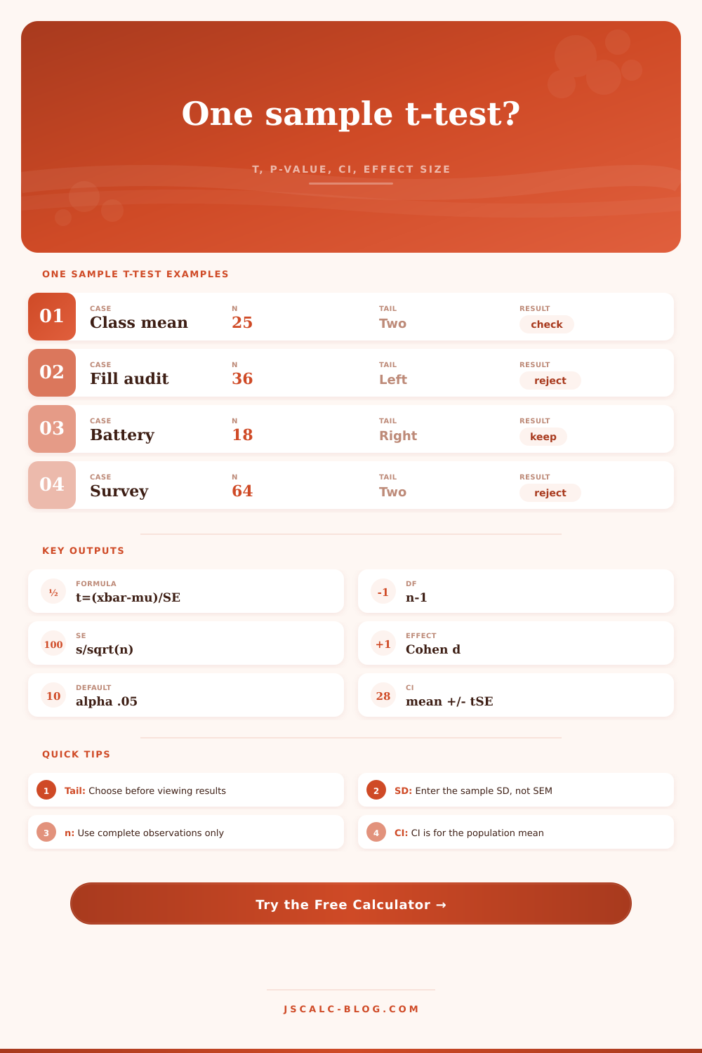
Test whether a sample mean differs from a hypothesized population mean using t = (sample mean - mu0) / (s / sqrt(n)), df = n - 1, p-value, confidence interval, effect size, and alpha decision.
📌Presets
Load a realistic one-sample test, then adjust the sample mean, hypothesized mean, standard deviation, sample size, tail, confidence level, and alpha.
Enter a sample mean, hypothesized mean, sample standard deviation, and sample size to calculate the test.
⚙Test Inputs
🔢Live Test Grid
📋Reference Tables
| One-sample setting | Typical input | Null mean cue | Tail choice | Output to report |
|---|---|---|---|---|
| Class score benchmark | Mean score, sample SD, n | Expected class average | Two-tailed if any change matters | t(df), p, CI, d |
| Manufacturing fill audit | Average fill volume | Label claim or target fill | Left-tailed for underfill | p-value and lower-side decision |
| Battery runtime test | Mean runtime in hours | Advertised runtime | Right or two-tailed by protocol | CI for mean runtime |
| Clinical marker screen | Mean lab marker value | Reference population mean | Two-tailed unless direction is pre-set | Effect size and assumption note |
| Sensor bias check | Mean reading error | Zero error target | Two-tailed for any bias | t statistic and CI around bias |
| Operations timing | Mean elapsed time | Service-level target | Left for faster, right for slower | alpha decision with practical size |
| Quantity | Formula | Uses df? | What it means |
|---|---|---|---|
| Mean difference | xbar - mu0 | No | Observed gap between sample mean and null mean. |
| Standard error | s / sqrt(n) | No | Estimated sampling spread of the sample mean. |
| t statistic | (xbar - mu0) / (s / sqrt(n)) | Yes | Distance from null in standard-error units. |
| Degrees of freedom | n - 1 | Yes | Controls the Student t distribution shape. |
| p-value | Tail area under t(df) | Yes | Evidence against H0 under the chosen alternative. |
| Mean CI | xbar +/- t* x SE | Yes | Plausible population mean interval at the selected confidence. |
| Cohen's d | (xbar - mu0) / s | No | Mean gap in sample-standard-deviation units. |
| df | 90% CI t* | 95% CI t* | 99% CI t* | Two-tail alpha .05 | One-tail alpha .05 |
|---|---|---|---|---|---|
| 5 | 2.015 | 2.571 | 4.032 | 2.571 | 2.015 |
🧮Formula Notes
Something feels different. Perhaps you suspect that your new manufacturing process is actualy faster. Or maybe the average test score in your class have changed from last semester. Whatever it is, you’ve got the data. You’ve got a benchmark to compare it with.
What’s missing? Is this a change that’s real, or is it simply the sort of random noise you get when you try to measure things? That’s where the one sample t-test comes into play. It allow you to determine whether signal is loud enough for you to be able to hear it over the background hum.
What is a One Sample T-Test?
To understand how this thing works, let’s take a quick peek under the hood. What does it do? It runs the numbers for you if you plug them into the calculator above (here). In short, it asks the following: Is there a difference between mean of your particular group compared to some guessed or known population mean?
To answer that, we want to know three things: 1) The number of observations 2) This is the average (or mean) of your sample. 3) This is the standard deviation of that same sample. Those three numbers tell the story of your data.
Most importantly, the standard deviation conveys how spread out your values are. A small standard deviation indicate that everyone in your sample is pretty similar; detecting a difference becomes relatively easy. A large standard deviation makes it more difficult for you to demonstrate your mean really differs from the benchmark if your data is all over the place. That’s where folks screw up. They only pay attention to the mean and not to the spread.
Then there are degrees of freedom. That’s just the sample size minus one. Why? Because smaller samples aren’t quite as good than bigger ones. To account for that uncertainty, the t-distribution has fatter tails than the normal distribution does. And the larger your sample size, the smaller those tails become. In other words, the t-distribution increasingly looks like textbook bell curve.
The page’s reference table makes this clear. It shows the critical values at varying sample sizes so that you can see how much they decrease as you collect more data. When your sample is small, you’re paying a premium for uncertainty.
The next question is what’s the correct choice for tail? Here again, think before looking. The default answer is a two-tailed test, which essentially asks “Is the mean different in either direction (higher or lower)?” If you don’t have a strong prior expectation of direction, this is a reasonable guess.
By contrast, a one-tailed test is more specific: it asks “Is the mean strictly greater then or strictly less than the benchmark value?” You get more statistical power to detect a difference in the chosen direction, but there’s a cost: if the difference turns out to go the opposite direction then you must accept the null hypothesis, even if the difference is large. This is not just a mathematical tradeoff, but a strategic one.
The test is run and you obtain a p-value. The p-value shows how likely it is that you would get your result (or something even more extreme) if the null hypothesis were true. A low p-value means that the difference you observe are unlikely to have occurred by chance alone. Although 0.05 is commonly used as a cutoff, this is an arbitrary cut in the sand.
For more context, there’s also the confidence interval. The confidence interval puts into perspective what possible values for the true population mean could be. If the value falls within your hypothesized mean then there is no claim of significance. Not only does the interval tell you whether or not you’re wrong, but it will tell you how wrong you may be.
And finally, we have effect size. Practical significance isn’t necessarily statistical significance. Perhaps you have a really huge sample and found some small difference between two adult-sized sofa that is statistically true. But is it meaningful? That depends on how much of a difference it is.
How big is the difference? The effect size is measured in standard deviation units using Cohen’s d. This gives you an idea about how large the difference is. It separates the important results from the unimportant ones, in ways that a raw p-value simply can’t do.
If you have a small sample and a large effect size, it may not be significant, but tell you there’s something worth looking into. If you have a huge sample size and tiny effect size, then yes, it will be significant, but maybe it doesn’t mean very much. Know the former, and you should of known the latter.
It makes you specific. It doesn’t allow you to say, “things are different.” You need to say what different is, how uncertain you can afford to be, and how large the difference has to be for it to matter.
It structures your hunch. It transforms your opinion into a conclusion. It is a conclusion based off numbers but framed by context.
How do you go from not knowing to knowing?